Greetings to everyone who’s enrolled in Habr’s Machine Learning course!
In the first two parts (1, 2), we practiced the initial/primary analysis of data with Pandas and making plots that allow us to draw conclusions about the data. Today we at last turn to machine learning. We’ll talk about tasks of machine learning and consider 2 simple approaches: decision trees and nearest neighbors method. We’ll also discuss how to use cross-validation to choose a model for specific data.
Напомним, что к курсу еще можно подключиться, дедлайн по 2 домашнему заданию – 13 марта 23:59.
1. [Первичный анализ данных с Pandas](https://habrahabr.ru/company/ods/blog/322626/) 2. [Визуальный анализ данных c Python](https://habrahabr.ru/company/ods/blog/323210/) 3. [Классификация, деревья решений и метод ближайших соседей](https://habrahabr.ru/company/ods/blog/322534/) 4. [Линейные модели классификации и регрессии](https://habrahabr.ru/company/ods/blog/323890/) 5. [Композиции: бэггинг, случайный лес](https://habrahabr.ru/company/ods/blog/324402/) 6. [Построение и отбор признаков. Приложения в задачах обработки текста, изображений и геоданных](https://habrahabr.ru/company/ods/blog/325422/) 7. Обучение без учителя: PCA, кластеризация, поиск аномалийPlan of this article:
- how to build a decision tree
- How a decision tree works with numerical data
- Main parameters of a decision tree
- DecisionTreeClassifier class in Scikit-learn
- Decision tree in a regression task
- Decision trees and kNN in churn rate prediction task
- Complex case in decision trees
- Decision trees and kNN in MNIST handwritten digits recognition task
- Complex case in kNN
You probably want to take right off to fight, but first let's talk about what kind of problem we are going to solve, and what is its place in the field of machine learning. Classical and general (and not that strict) definition of machine learning is as follows (T. Mitchell "Machine learning", 1997): A computer program > is said to learn to solve some problem of class T if its performance according to the P metric , improves with accumulating experience E.
Further, in the various settings T, P, and E can refer to completely different things. Among the most popular tasks T in machine learning are:
- classification of the object to one of the categories on the basis of its features
- regression - prediction of numerical variable/target on the basis of its other features
- clustering - partition of objects into groups based on the features of these objects so that the objects within the groups were similar to each other, and objects from different groups were different
- anomaly detection - search for objects that are "greatly dissimilar" to the rest of the sample or to some group of objects
- and many more, more specific. A good overview is given in the "Deep Learning" (Ian Goodfellow, Yoshua Bengio, Aaron Courville, 2016) book, chapter "Machine Learning basics" (by Ian Goodfellow, Yoshua Bengio, Aaron Courville, 2016)
**Experience E ** means data (can't go anywhere without it), and depending on that machine learning algorithms can be divided into those that are trained with the teacher (supervised learning) and those that are trained without a teacher (unsupervised learning). In unsupervised learning tasks, one has a sample consisting of objects described by a set of features. In supervised learning problems, there's also a target variable known for each object of a training set - that is, in fact, what we would like to predict for other objects outside the training set.
Classification and regression are supervised learning problems. As an example, we propose the problem of credit scoring: based on data that credit institution has accumulated about its clients, we want to predict loan default. Here, experience E for the algorithm is the available training data: a set of objects (people), each of which is characterized by a set of features (such as age, salary, type of loan, past loan defaults, etc.), and a target variable. If the target variable is just a fact of loan default (1 or 0, ie the bank knows who of its clients returned the loan and who didn't), then this is (binary) classification problem. If you know by how much time the client has overdued the loan repayment and want to predict the same thing for new customers, it will be the regression problem.
Finally, the third abstraction in the definition of machine learning is a metric of algorithm's performance evaluation P. Such metrics differ for different problems and algorithms, and we'll talk about them as we learn new algorithms.For now let's just say that the simplest metric of classification algorithm quality is the proportion of correct answers - accuracy; do not confuse it with precision) - that is simply the proportion of correct predictions of the algorithm on the test set.
Next we'll talk about two supervised learning problems: classification and regression.
Let's start the review of classification and regression methods with the most popular one - a decision tree. Decision trees are used in everyday life in various fields of human activity, sometimes very far from machine learning. We can call visual instructions of what to do in a situation a decision tree. Here is an example from the field of consulting the scientific staff of the Institute. Higher School of Economics publishes information diagrams to make the lives of its employees easier. Here's a snippet of instructions for the publication of scientific articles on the portal of the Institute.
In terms of machine learning can be said that this is an elementary classifier that determines the form of the publication on the portal (book, article, chapter of the book, preprint, publication in the "Higher School of Economics and the media") on several factors: the type of publication (book, pamphlet, paper and etc.), type of publication, which published an article (scientific journal, proceedings, etc.) and others.
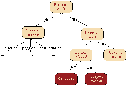
Decision tree is often a generalization of the experts experience, means of knowledge transfer to prospective employees or a model of the business process. For example, before the introduction of scalable machine learning algorithms, the credit scoring problem in the banking sector was solved by experts. The decision to grant a loan to the borrower was taken on the basis of some intuitively (or empirically) derived rules that can be represented as a decision tree.
In this case, we can say that binary classification problem is solved (the target class has two values: "To issue a loan" and "To deny") on the grounds of "Age", "The presence of the house", "Income" and "Education".
The decision tree as a machine learning algorithm is essentially the same thing: incorporation of the logical rules of the form "feature $inline$a$inline$ value is less than $inline$x$inline$ and feature $inline$b$inline$ value is less than $inline$y$inline$ ... => Category 1" into the "tree"-like data structure. The great advantage of decision trees is that they are easily interpretable and human understandable. For example, using the above scheme one can explain the borrower why he was denied a loan. Like, because he doesn't own a house and his income is less than 5,000. As we'll see, many other models, although more accurate, do not have this property and can be regarded more as a "black box" where we put the data and received an answer. Due to such "understandability" and similarity to human decision-making (you can easily explain your model to the boss), decision trees have gained immense popularity. One of the representatives of this group of classification methods, C4.5, is even considered the first in the list of 10 the best data mining algorithms ( "top 10 algorithms in data mining", Knowledge and Information Systems, 2008. PDF)).
In the example of credit scoring, we saw that the decision to grant a loan was taken on the basis of age, tenure, income and other variables. But what variable to choose first? For that sake, let's consider a simpler example where all the variables are binary.
Here we can recall the game of "20 Questions" which is often referred to in the introduction to the decision trees. Surely everyone played it. One person thinks of a celebrity, and the other tries to guess by asking questions that you can answer only "Yes" or "No" to (we'll omit the options "don't know" and "can't say"). What question the guesser will ask first? Of course, the one that will reduce the number of the remaining options the most. For example, the question "Is this Angelina Jolie?" in case of a negative response will leave more than 7 billion options for further sorting (a little smaller, of course, not every person is a celebrity, but still a lot). But the question "Is this a woman?" cuts off about half the celebrities. That is, "sex" feature separates dataset of people much better than features "Angelina Jolie", "Hispanic nationality" or "loves football." This intuitively corresponds to the notion of information gain based on entropy.
Shannon entropy is defined for a system with N possible states as follows:
where $inline$p_i$inline$ is the probability of finding the system in the $inline$i$inline$-th state. This is a very important concept used in physics, information theory and other areas. Let's omit the introduction prerequisites (combinatorial and information-theoretic) of this concept and note that, intuitively, entropy corresponds to the degree of chaos in the system. The higher the entropy, the less ordered the system and vice versa. This will help us to formalize the "effective division of data" that we mentioned t in the context of the "20 Questions" game.
To illustrate how the entropy will help us identify good features for building a decision tree, let's look at a toy example from the "Entropy and decision trees" paper. We'll predict the color of the ball by its coordinates. Of course, this has nothing to do with real life, but it will show us how entropy is used to construct a decision tree.
Here are 9 blue balls and 11 yellow. If we randomly pull out a ball, then with probability $inline$p_1=\frac{9}{20}$inline$ it'll be blue and with probability $inline$p_2=\frac{11}{20}$inline$ - yellow. Hence, the entropy of the state $inline$S_0 = -\frac{9}{20}\log_2{\frac{9}{20}}-\frac{11}{20}\log_2{\frac{11}{20}} \approx 1$inline$. Of course, this value by itself doesn't tell us much. Now let's see how the entropy will change if we break the balls into two groups: with the coordinate less than or equal to 12 and greater than 12.
The left group has 13 balls, 8 of which are blue and 5 are yellow. The entropy of this group is $inline$S_1 = -\frac{5}{13}\log_2{\frac{5}{13}}-\frac{8}{13}\log_2{\frac{8}{13}} \approx 0.96$inline$. The right group has 7 balls, 1 of them is blue, 6 are yellow. Entropy of the right group is $inline$S_2 = -\frac{1}{7}\log_2{\frac{1}{7}}-\frac{6}{7}\log_2{\frac{6}{7}} \approx 0.6$inline$. As you can see, the entropy has decreased in both groups compared with the initial state, although not that much in the left group. Since the entropy is in fact the degree of chaos (or uncertainty) in the system, reducing the entropy is called information gain. Formally, information gain (IG) in division of the data on the basis of the variable $inline$Q$inline$ (in this example, it's a variable of "$inline$x \leq 12$inline$") is defined as
It turns out that dividing the balls into two groups according to the feature "coordinate less than or equal to 12" gives us more orderly system than at the beginning. Let's continue division into groups until the balls in each group are the same color.
For the right group it only took one extra partition on the grounds of "coordinate less than or equal to 18", while for the left one we needed three more. Apparently, entropy of a group of with the balls of the same color is equal to 0 (
We can make sure that the tree built in the previous example is in a sense optimal: it took only 5 "questions" (conditions on the variable $inline$x$inline$), to "fit" a decision tree to the training set, ie to make the tree correctly classify any training example. Under other split conditions the tree will get deeper.
At the heart of the popular algorithms for decision tree construction, such as ID3 and C4.5, lies the principle of greedy maximization of the information gain: on each step, the the algorithm chooses such variable that during split gives the greatest information gain. Then the procedure is repeated recursively until the entropy is zero or of some small value (if the tree is not fitted perfectly to the training set in order to avoid overfitting). Different algorithms use different heuristics for "early stop" or "cut-off" to avoid the construction of overfitted tree.
def build(L):
    create node t
    if the stopping criterion is True:
        assign a predictive model to t
    else:
        Find the best binary split L = L_left + L_right
        t.left = build(L_left)
        t.right = build(L_right)
return t We figured how the concept of entropy allows to formalize an idea of the partition in the tree. But this is only a heuristic, and there exist others:
- Gini uncertainty(Gini impurity): $inline$G = 1 - \sum\limits_k (p_k)^2$inline$. Maximizing this criterion can be interpreted as the maximization of the number of pairs of objects of the same class that are in the same subtree. Read more about this (as well as about many other things) in Evgeny Sokolov repository. Not to be confused with the Gini index! More about this confusion in Alexander Dyakonov post
- Error of classification (misclassification error): $inline$E = 1 - \max\limits_k p_k$inline$
In practice, misclassification error is almost never used, and Gini uncertainty and information gain work quite the same.
In the case of binary classification problem ($inline$p_+$inline$ - the probability of an object having a label +) entropy and Gini uncertainty take the following form:
If we plot these two functions against the argument $inline$p_+$inline$, we'll see that the entropy plot is very close to the doubled plot of Gini uncertainty, and therefore, in practice, these two criteria are almost identical.
```python from __future__ import division, print_function # turn off Anaconda warnings import warnings warnings.filterwarnings('ignore') import numpy as np import pandas as pd import pylab as plt %matplotlib inline import seaborn as sns from matplotlib import pyplot as plt ``` ```python plt.rcParams['figure.figsize'] = (6,4) xx = np.linspace(0,1,50) plt.plot(xx, [2 * x * (1-x) for x in xx], label='gini') plt.plot(xx, [4 * x * (1-x) for x in xx], label='2*gini') plt.plot(xx, [-x * np.log2(x) - (1-x) * np.log2(1 - x) for x in xx], label='entropy') plt.plot(xx, [1 - max(x, 1-x) for x in xx], label='missclass') plt.plot(xx, [2 - 2 * max(x, 1-x) for x in xx], label='2*missclass') plt.xlabel('p+') plt.ylabel('criterion') plt.title(Criteria of quality as a function of p+ (binary classification)') plt.legend(); ```Let's consider the example of the application of decision trees from Scikit-learn library to synthetic data. Two classes will be generated from two normal distributions with different means.
```python # first class np.seed = 7 train_data = np.random.normal(size=(100, 2)) train_labels = np.zeros(100)train_data = np.r_[train_data, np.random.normal(size=(100, 2), loc=2)] train_labels = np.r_[train_labels, np.ones(100)]
</spoiler>


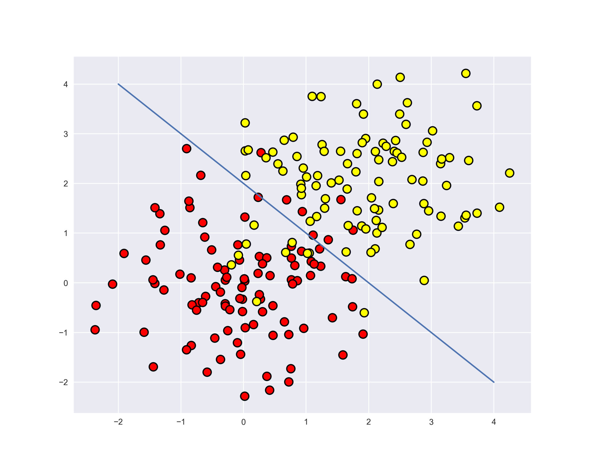
Let's plot the data. Informally, the classification problem in this case is to build some "good" boundary separating two classes (red dots from yellow). Machine learning in this case boils down to, roughly speaking, choosing a good dividing border. Maybe straight line will be too simple of a boundary, and some complex curve enveloping each red dot will be too complex, so that we'll make a lot of mistakes on the new examples from the same distribution that the training set came from. Intuition suggests that on the new data some smooth border between the two classes, or even just a straight line (in the $inline$n$inline$-dimensional case, a hyperplane). will work better.

<spoiler title="Drawing picture">
```python

plt.rcParams['figure.figsize'] = (10,8)
plt.scatter(train_data[:, 0], train_data[:, 1], c=train_labels, s=100,
cmap='autumn', edgecolors='black', linewidth=1.5);
plt.plot(range(-2,5), range(4,-3,-1));
Let's try to separate these two classes by training a decision tree. We will use max_depth parameter that limits the depth of the tree. Let's visualize the resulting boundary separating classes.
def get_grid(data): x_min, x_max = data[:, 0].min() - 1, data[:, 0].max() + 1 y_min, y_max = data[:, 1].min() - 1, data[:, 1].max() + 1 return np.meshgrid(np.arange(x_min, x_max, 0.01), np.arange(y_min, y_max, 0.01))
clf_tree = DecisionTreeClassifier(criterion='entropy', max_depth=3, random_state=17)
clf_tree.fit(train_data, train_labels)
xx, yy = get_grid(train_data) predicted = clf_tree.predict(np.c_[xx.ravel(), yy.ravel()]).reshape(xx.shape) plt.pcolormesh(xx, yy, predicted, cmap='autumn') plt.scatter(train_data[:, 0], train_data[:, 1], c=train_labels, s=100, cmap='autumn', edgecolors='black', linewidth=1.5);
</spoiler>


<img align='center' src='https://habrastorage.org/files/560/d97/0ca/560d970caaf749fda34bd8417160ed7e.png'><br>


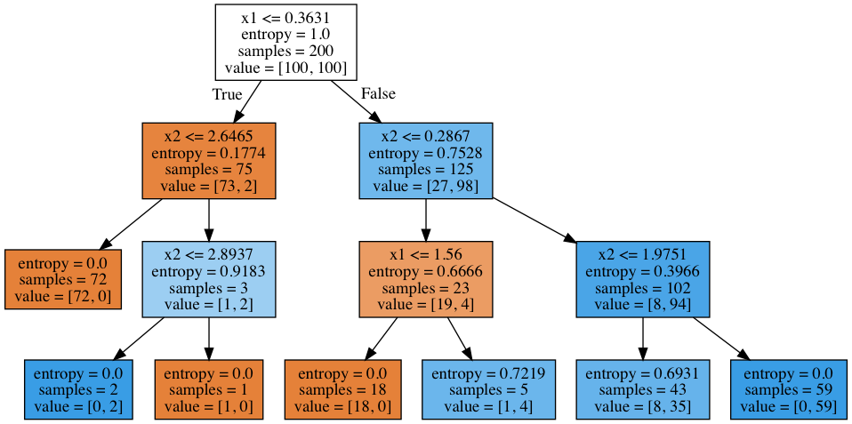
And how does the tree itself look? We see that the tree "cuts" the space into 7 rectangles (tree has 7 leaves). In each such rectangle, tree will make constant predictions according to the majority class of objects inside it.

<spoiler title="The code to display a tree">
```python
# use .dot format to visualize tree
from sklearn.tree import export_graphviz
export_graphviz(clf_tree, feature_names=['x1', 'x2'],
out_file='../../img/small_tree.dot', filled=True)
# for this we’ll need pydot library (pip install pydot)
!dot -Tpng '../../img/small_tree.dot' -o '../../img/small_tree.png'
How to "read" a tree?
In the beginning there were 200 objects, 100 of one class and 100 of the other. Entropy of the initial state was maximal - 1. Then the partition of objects into 2 groups was made by comparing value of $inline$x_1$inline$ with $inline$0.3631$inline$ (find this part of the border in the picture above, before the tree). With that, the entropy of both left and right groups of objects decreased. And so on, the tree is constructed up to a depth of 3. In this visualization, the more objects of one class, the darker the orange color of the vertex and vice versa: the more objects of the second class, the darker the blue color. At the beginning, the number of objects from two classes is equal, so the root node of the tree is white.
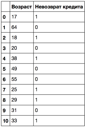
Suppose we have a numeric variable "Age" in the dataset that has a lot of unique values. Decision Tree will look for the best (according to some criterion of the information gain type) split by checking the binary attributes such as "Age <17", "Age <22.87", etc. But what if there are too many such "cuts"? What if there is another quantitative variable, "salary", and it, too, can be "cut" in many ways? It turns out to be too many binary attributes to select from on each step of the tree construction. To resolve this problem, heuristics are usually used to limit the number of thresholds which we compare the quantitative variable to.
Let's consider a toy example. Suppose we have the following dataset:
Let's sort it by age in ascending order.
Let's train a decision tree on this data (without depth restrictions) and look at the it.
age_tree = DecisionTreeClassifier(random_state=17)
age_tree.fit(data['Возраст'].values.reshape(-1, 1), data['Невозврат кредита'].values)

export_graphviz(age_tree, feature_names=['Возраст'],
out_file='../../img/age_tree.dot', filled=True)
!dot -Tpng '../../img/age_tree.dot' -o '../../img/age_tree.png'
We see that the tree used 5 values to compare the age to: 43.5, 19, 22.5, 30 and 32 years. If you look closely, these are exactly the mean values between the ages at which the target class "changes" from 1 to 0 or vice versa. That's a complex sentence, so here's an example: 43.5 is an average between 38 and 49 years; the customer who was 38 years failed to return the loan, and the one who was 49 did return the loan. Similarly, 19 years is an average between 18 and 20 years. That is, a tree looks for the values at which the target class changes its value as a threshold for "cutting" quantitative variable.
Think why it makes no sense in this case to consider a feature of "Age <17.5".
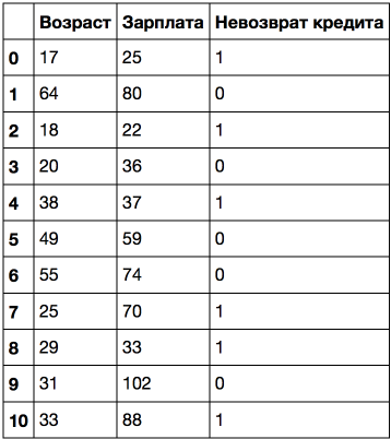
Let's consider a more complex example and add "Salary" variable (thousand rubles/month).
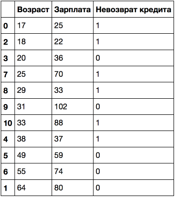
If we sort by age, the target class ( "loan default") changes (from 1 to 0 or vice versa) 5 times. And if we sort by salary, it changes 7 times. How the tree will now choose variables? Let's see.
age_sal_tree = DecisionTreeClassifier(random_state=17)
age_sal_tree.fit(data2[['Возраст', 'Зарплата']].values, data2['Невозврат кредита'].values);

export_graphviz(age_sal_tree, feature_names=['Возраст', 'Зарплата'],
out_file='../../img/age_sal_tree.dot', filled=True)
!dot -Tpng '../../img/age_sal_tree.dot' -o '../../img/age_sal_tree.png'
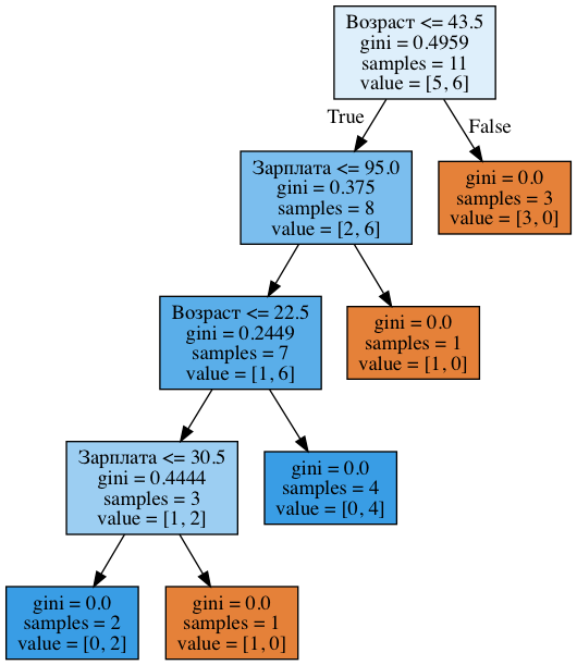
We see that the tree involves both age and salary based partitions. Moreover, the thresholds for feature comparisons are 43.5 and 22.5 years for age, and 95 and 30.5 thousand rubles/month for salary. And again, we can notice that 95 thousand is the average between 88 and 102, while a person with a salary of 88 proved to be "bad", and the one with 102 - "good". The same goes for 30.5 thousand. That is only a few values for comparison of age and salary were searched, not all of them. And why the tree turned out to have exactly these features? Because they gave better partitioning (according to Gini uncertainty).
Conclusion: the simplest heuristics for handling quantitative variables in a decision tree is to sort it in ascending order and check only those thresholds where the value of the target variable changes. It does not sound very strict, but I hope I have conveyed the meaning with the help of toy examples.
Further, when there are many quantitative variables in data, and each has a lot of unique values, not all thresholds described above are selected, but only top-N that give maximum gain according to the same criterion. That is, in fact, for each threshold a tree of depth 1 is constructed, then the entropy (or Gini uncertainty) is computed, and only best thresholds are selected for comparison.
Here's an illustration: if we make the split by "Salary
More examples of discretisation of quantitative variables can be found in posts like this or this.One of the most prominent scientific papers on the subject is "On the handling of continuous-valued attributes in decision tree generation" (UM Fayyad. KB Irani, "Machine Learning", 1992).
Technically, you can build a decision tree of such depth that each leaf has exactly one object. But this is not common in practice (if only one tree is built) because such a tree will be overfitted, or too tuned to the training set, and will not work well to predict the new data.Somewhere at the bottom of the tree, in a great depth, there will appear partitions based on less important features (for example, whether a client came from Saratov or Kostroma). If we exaggerate, it may happen that of all four clients who came to the bank for a loan in green trousers, nobody has returned the loan. But we don't want our classification model to generate such specific rules.
There are two exceptions, the situations when the trees are built to the maximum depth:
- Random Forest (composition of many trees) averages the responses of trees that are built up to the maximum depth (we'll talk later on why you should do so)
- Pruning trees. In this approach, the tree is first constructed to the maximum depth, then gradually, from the bottom up, some nodes of the tree are removed by comparing the quality of the tree with this partition and without it (comparison is performed using cross-validation, on which below). More details can be found in materials in Evgeny Sokolov repository.
The picture below is an example of dividing border built by an overfitted tree.
The main ways to deal with overfitting in case of decision trees are:
- artificial limitation of the depth or the minimum number of objects in the leaf: the construction of a tree just stops at some point;
- pruning the tree
The main parameters of the sklearn.tree.DecisionTreeClassifier class:
max_depth– the maximum depth of the treemax_features- the maximum number of features to search for the best partition (this is necessary because with a large number of variables it'll be "expensive" to look for the best (according to the information gain-type criterion) partition among all variables)min_samples_leaf– the minimum number of objects in a leaf.This parameter has a clear interpretation: for example, if it is equal to 5, the tree will produce only those classifying rules that are true for at least 5 objects
The parameters of tree need to be set depending on the input data, and it is usually done with the help of cross-validation, more on it below.
When forecasting the quantitative variable, the idea of the tree construction remains the same, but the quality criteria changes:
- The dispersion around the mean:
$inline$ \Large D = \frac{1}{\ell} \sum\limits_{i =1}^{\ell} (y_i - \frac{1}{\ell} \sum\limits_{i =1}^{\ell} y_i)^2,$inline$ where$inline$ \ell$inline$ is the number of objects in the leaf, $inline$y_i$inline$ is value of the target variable.Simply put, by minimizing the variance around the mean, we look for variables that divide the training set so that the values of the target variable in each leaf are roughly equal.
Let's generate some data distributed around the function $inline$f(x) = e^{-x ^ 2} + 1.5 * e^{-(x - 2) ^ 2}$inline$ with some noise, then train the tree on it and show what forecasts it makes.
```python n_train = 150 n_test = 1000 noise = 0.1def f(x): x = x.ravel() return np.exp(-x ** 2) + 1.5 * np.exp(-(x - 2) ** 2)
def generate(n_samples, noise):
X = np.random.rand(n_samples) * 10 - 5
X = np.sort(X).ravel()
y = np.exp(-X ** 2) + 1.5 * np.exp(-(X - 2) ** 2) +
np.random.normal(0.0, noise, n_samples)
X = X.reshape((n_samples, 1))
return X, y
X_train, y_train = generate(n_samples=n_train, noise=noise) X_test, y_test = generate(n_samples=n_test, noise=noise)
from sklearn.tree import DecisionTreeRegressor
reg_tree = DecisionTreeRegressor(max_depth=5, random_state=17)
reg_tree.fit(X_train, y_train) reg_tree_pred = reg_tree.predict(X_test)
plt.figure(figsize=(10, 6)) plt.plot(X_test, f(X_test), "b") plt.scatter(X_train, y_train, c="b", s=20) plt.plot(X_test, reg_tree_pred, "g", lw=2) plt.xlim([-5, 5]) plt.title("Decision tree regressor, MSE = %.2f" % np.sum((y_test - reg_tree_pred) ** 2)) plt.show()
</spoiler>
<img align='center' src='https://habrastorage.org/files/856/c8b/9ad/856c8b9ad9094250a9d23e91e6f74e97.png'><br>
We see that the decision tree approximates the relationship in the data by piecewise constant function.
# Nearest Neighbors Method
Nearest neighbors method (k Nearest Neighbors, or kNN) is another very popular classification method that is also sometimes used in regression problems. This is, along with the decision tree, one of the most comprehensible approaches to classification. Intuitively, the essence of the method is as follows: you are like the neighbors around you. Formally, the basis of the method is the compactness hypothesis: if the distance between the examples is measured well enough, then similar examples are much more likely to belong to the same class, than to different ones.
According to the nearest neighbors method, the test case (green ball) is classified as "blue" rather than "red".
<img src='https://habrastorage.org/files/4b8/000/4ab/4b80004ab2414944802677e2e1cb1b76.png' align='center'><br>
For example, if you don't know what type of product to specify in the ad for of Bluetooth-headset, you can find 5 similar headsets, and if 4 of them are tagged as "accessories" and only one as "Technology" then common sense will tell you to tag your ad also with "Accessories" category.
To classify each object from the test set, one needs to perform the following operations step by step:
- Calculate the distance to each of the objects of the training set
- Select $inline$k$inline$ objects from the training set with the minimal distance to them
- The class of the test object will be the most frequent class among the $inline$k$inline$ nearest neighbors
The method adapts quite easily for the regression problem: on step 3, it returns not the class, but the number - mean (or median) of the target variable among neighbors.
A notable feature of this approach is its laziness. This means that calculations start only when a test case needs to be classified, and in advance, in the presence of only training examples, no model is constructed. That's a distinction from, say, a decision tree that we discussed earlier. The tree is constructed at the very beginning based on the training set, and then classification of test cases occurs relatively quickly.
It should be noted that the method of nearest neighbors is a well-studied approach (in machine learning, statistics and econometrics more is known probably only about linear regression). For the method of nearest neighbors, there are many important theorems claiming that on the "endless" datasets it's the optimal method of classification. The authors of the classic book "The Elements of Statistical Learning" consider kNN to be theoretically ideal algorithm, which application is only limited to the computing power and curse of dimensionality.
### Nearest Neighbors Method in Real Applications
- kNN alone can serve as a good starting point (baseline) in the solution of a problem;
- In Kaggle competitions, kNN is often used for the construction of meta-features (kNN predictions are input to the other models) or in stacking/blending;
- The idea of the nearest neighbor also extends to other tasks, for example, in a simple recommendation systems, the initial decision could be a recommendation of a product (or service), popular among the *closest neighbors* of the person who we want to make a recommendation;
- In practice, for large datasets approximate methods of search for nearest neighbors are often used. [Here's](https://www.youtube.com/watch?v=UUm4MOyVTnE) lecture by Artem Babenko about efficient algorithms for nearest neighbors search among billions of objects in high dimensional space (image search).There also exist open source libraries that implement these algorithms, thanks to Spotify company for its library [Annoy](https://github.com/spotify/annoy).
Quality of classification/regression implemented with kNN depends on several parameters:
- the number of neighbors
- the measure of distance between the objects (people often use Hamming, Euclidean, cosine and Minkowski distances). Note that using most of the metrics requires data to be scaled. Relatively speaking, it's needed so that a "salary" variable with the range up to 100 thousand wouldn't make a greater contribution to the distance than the "Age" variable with values up to 100.
- weights of neighbors (test case's neighbors may contribute with different weights, for example, the further the sample, the lower the coefficient for its "voice")
### Class KNeighborsClassifier in Scikit-learn
The main parameters of the class sklearn.neighbors.KNeighborsClassifier:
- weights: "uniform" (all weights are equal), "distance" (the weight is inversely proportional to the distance from the test case) or other user-defined function
- algorithm (optional): "brute", "ball_tree ", "KD_tree", or "auto". In the first case, the nearest neighbors for each test case are computed by a grid search over a training set. In the second and third cases the distances between the examples are stored in the tree which accelerates finding nearest neighbors. In you set this parameter to "auto", the right way to find the neighbors will be chosen automatically based on the training set.
- leaf_size (optional): threshold for switching to a grid search in case of BallTree or KDTree choice for finding neighbors
- metric: "minkowski", "manhattan ", "euclidean", "chebyshev" and other
# The Choice of Model Parameters and Cross-Validation
The main task of learning algorithms is to be able to *generalize*, that is, work well on the new data.Since we can't right away check the model performance on the new data ('cause we need to make a prediction for them, that is we don't know the true values of the target variable for them), it is necessary to sacrifice a small portion of the data to check the quality of the model on it.
Чаще всего это делается одним из 2 способов:
Most often this is done in one of two ways:
- putting aside a part of the dataset (*held-out/hold-out set*).In this approach, we reserve a fraction of the training set (typically from 20% to 40%), train the model on the rest of the data (60-80% of the original set) and compute some performance metric for the model (for example, the most simple one - the proportion of correct answers in the classification problem) on the hold-out set.
- *cross-validation*. The most frequent case here is K-fold cross-validation
<img align='center' src='https://habrastorage.org/files/b1d/706/e6c/b1d706e6c9df49c297b6152878a2d03f.png'><br>
Here, the model is trained $inline$K$inline$ times on different ($inline$K-1$inline$) subsets of the original dataset (in white), and checked on one subset (each time a different one, in orange).
We obtained $inline$K$inline$ model quality assessments that are usually averaged to give an average quality of classification/regression on cross-validation.
Cross-validation provides a better assessment of the model quality on the new data compared to the hold-out set. However, cross-validation of computationally expensive if you have a lot of data.
Cross-validation is a very important technique in machine learning (also used in statistics and econometrics). Model hyperparameters are selected with its help, models are compared with each other, the usefulness of the new features is evaluated, etc. More details can be found, for example, [here](https://sebastianraschka.com/blog/2016/model-evaluation-selection-part1.html) by Sebastian Raschka or in any classic textbook on machine (statistical) learning.
# Examples of Application
### Decision trees and nearest neighbors method in the problem of customer churn prediction for telecom operator
Let's read data into DataFrame and preprocess it. Let's store States in a separate Series object for now and remove it from the dataframe. We'll train the first model without state, then we'll see if they help.
<spoiler title="Reading and preprocessing of data">
```python
df = pd.read_csv('../../data/telecom_churn.csv')
df['International plan'] = pd.factorize(df['International plan'])[0]
df['Voice mail plan'] = pd.factorize(df['Voice mail plan'])[0]
df['Churn'] = df['Churn'].astype('int')
states = df['State']
y = df['Churn']
df.drop(['State', 'Churn'], axis=1, inplace=True)
Let's allocate 70% of the set (X_train, y_train) for training and 30% will be a hold-out set (X_holdout, y_holdout). Hold-out set will not in any way be involved in tuning the parameters of the models. We'll use it in the end, after this tuning, to assess the quality of the resulting model. Let's train 2 models - decision tree and kNN, for now we don't know what parameters are good, so we'll use some random ones: the tree depth 5, the number of nearest neighbors 10.
```python from sklearn.model_selection import train_test_split, StratifiedKFold from sklearn.neighbors import KNeighborsClassifierX_train, X_holdout, y_train, y_holdout = train_test_split(df.values, y, test_size=0.3, random_state=17)
tree = DecisionTreeClassifier(max_depth=5, random_state=17) knn = KNeighborsClassifier(n_neighbors=10)
tree.fit(X_train, y_train) knn.fit(X_train, y_train)
</spoiler>


We'll assess predictions quality with a simple metric - the proportion of correct answers. Let's make prediction for the hold-out set. Decision Tree did better: percentage of correct answers is about 94% against 88% in kNN. But that's with random parameters.

<spoiler title="Code for model evaluation">
```python
from sklearn.metrics import accuracy_score

tree_pred = tree.predict(X_holdout)
accuracy_score(y_holdout, tree_pred) # 0.94
knn_pred = knn.predict(X_holdout)
accuracy_score(y_holdout, knn_pred) # 0.88
Now let's configure the parameters of the tree on cross-validation. We'll tune the maximum depth and the maximum number of features used at each split. Here's the essence of how the GridSearchCV works: for each unique pair of values of max_depth and max_features, there will be held 5-fold cross-validation, and then the best combination of parameters will be selected.
tree_params = {'max_depth': range(1,11),
'max_features': range(4,19)}
tree_grid = GridSearchCV(tree, tree_params,
cv=5, n_jobs=-1,
verbose=True)tree_grid.fit(X_train, y_train)Лучшее сочетание параметров и соответствующая средняя доля правильных ответов на кросс-валидации:
tree_grid.best_params_{'max_depth': 6, 'max_features': 17}
tree_grid.best_score_0.94256322331761677
accuracy_score(y_holdout, tree_grid.predict(X_holdout))0.94599999999999995
Теперь попробуем настроить число соседей в алгоритме kNN.
from sklearn.pipeline import Pipeline
from sklearn.preprocessing import StandardScalerknn_pipe = Pipeline([('scaler', StandardScaler()), ('knn', KNeighborsClassifier(n_jobs=-1))])knn_params = {'knn__n_neighbors': range(1, 10)}knn_grid = GridSearchCV(knn_pipe, knn_params,
cv=5, n_jobs=-1,
verbose=True)knn_grid.fit(X_train, y_train)knn_grid.best_params_, knn_grid.best_score_({'knn__n_neighbors': 7}, 0.88598371195885128)
accuracy_score(y_holdout, knn_grid.predict(X_holdout))0.89000000000000001
In this example, the tree proved to be better than the nearest neighbors method: 94.2% of correct answers on cross-validation and 94.6% on the hold-out set vs. 88.6%/89% for the kNN. Moreover, in this problem tree performs very well, and even random forest (let's think of it for now as a bunch of trees that are for some reason working better together) in this example shows not much better proportion of correct answers (95.1% on cross-validation and 95.3% on hold-out set), but trains much longer.
```python from sklearn.ensemble import RandomForestClassifierforest = RandomForestClassifier(n_estimators=100, n_jobs=-1, random_state=17) print(np.mean(cross_val_score(forest, X_train, y_train, cv=5))) # 0.949
```python
forest_params = {'max_depth': range(1,11),
'max_features': range(4,19)}
forest_grid = GridSearchCV(forest, forest_params,
cv=5, n_jobs=-1,
verbose=True)forest_grid.fit(X_train, y_train)forest_grid.best_params_, forest_grid.best_score_ # ({'max_depth': 9, 'max_features': 6}, 0.951)accuracy_score(y_holdout, forest_grid.predict(X_holdout)) # 0.953Let's draw the resulting tree. Due to the fact that it is not entirely a toy example (maximum depth is 6), the picture is not that small, but you can "walk" over the tree if you click on picture.
```python export_graphviz(tree_grid.best_estimator_, feature_names=df.columns, out_file='../../img/churn_tree.dot', filled=True) !dot -Tpng '../../img/churn_tree.dot' -o '../../img/churn_tree.png' ```To continuing the discussion of the pros and cons of discussed methods, let's consider a very simple example of a classification problem, where a tree performs well but does it in somewhat "complicated" manner. Let's create a set of points on a plane (2 features), each point will be one of two classes (+1 for red, or -1 for yellow). If you look at it as a classification problem, it seems very simple - the classes are separated by a line.
```python def form_linearly_separable_data(n=500, x1_min=0, x1_max=30, x2_min=0, x2_max=30): data, target = [], [] for i in range(n): x1, x2 = np.random.randint(x1_min, x1_max), np.random.randint(x2_min, x2_max)if np.abs(x1 - x2) > 0.5: data.append([x1, x2]) target.append(np.sign(x1 - x2)) return np.array(data), np.array(target)
X, y = form_linearly_separable_data()
plt.scatter(X[:, 0], X[:, 1], c=y, cmap='autumn', edgecolors='black');
</spoiler>
<img align='center' src='https://habrastorage.org/files/efe/630/812/efe6308122d24681a635fdf8a6d361d9.png'><br>
However, the border that decision tree builds is too complicated, and the tree itself is very deep. Also, imagine how bad the tree will generalize to the space beyond presented $inline$30 \times 30$inline$ square that frames the training set.
<spoiler title="Code to draw the dividing surface that is built by the tree">
```python
tree = DecisionTreeClassifier(random_state=17).fit(X, y)
xx, yy = get_grid(X, eps=.05)
predicted = tree.predict(np.c_[xx.ravel(), yy.ravel()]).reshape(xx.shape)
plt.pcolormesh(xx, yy, predicted, cmap='autumn')
plt.scatter(X[:, 0], X[:, 1], c=y, s=100,
cmap='autumn', edgecolors='black', linewidth=1.5)
plt.title('Easy task. Decision tree compexifies everything');
We got this overly complex construction, although the solution (good separating surface) is just a straight line $inline$x_1 = x_2$inline$.
```python export_graphviz(tree, feature_names=['x1', 'x2'], out_file='../../img/deep_toy_tree.dot', filled=True) !dot -Tpng '../../img/deep_toy_tree.dot' -o '../../img/deep_toy_tree.png' ```The method of one nearest neighbor does better than tree here, but still not as good as a linear classifier (our next topic).
```python knn = KNeighborsClassifier(n_neighbors=1).fit(X, y)xx, yy = get_grid(X, eps=.05) predicted = knn.predict(np.c_[xx.ravel(), yy.ravel()]).reshape(xx.shape) plt.pcolormesh(xx, yy, predicted, cmap='autumn') plt.scatter(X[:, 0], X[:, 1], c=y, s=100, cmap='autumn', edgecolors='black', linewidth=1.5); plt.title('Easy task, kNN. Not bad');
</spoiler>
<img align='center' src='https://habrastorage.org/files/998/ad6/80c/998ad680c23e482d90193066059ec94c.png'><br>
### Decision Trees and kNN in Task of MNIST Handwritten Digits Recognition
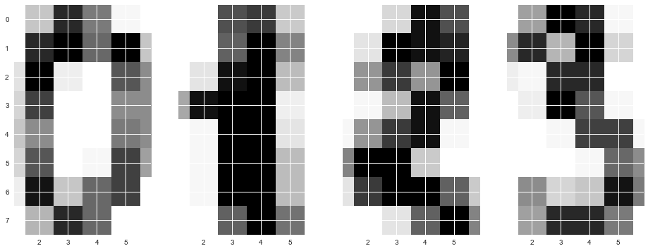
Now let's look how these 2 algorithms perform in the real-world problem. We'll use the "embedded" in `sklearn` data on handwritten digits.This problem is an example when kNN works surprisingly well.
Pictures here are 8x8 matrices (intensity of white color for each pixel). Then each such matrix is "unfolded" into a vector of length 64, and we obtain a feature description of an object.
Let's draw some handwritten digits, we see that they are guessable.
<spoiler title="Loading data and drawing a few digits">
```python
from sklearn.datasets import load_digits
data = load_digits()
X, y = data.data, data.target
X[0,:].reshape([8,8])
array([[ 0., 0., 5., 13., 9., 1., 0., 0.], [ 0., 0., 13., 15., 10., 15., 5., 0.], [ 0., 3., 15., 2., 0., 11., 8., 0.], [ 0., 4., 12., 0., 0., 8., 8., 0.], [ 0., 5., 8., 0., 0., 9., 8., 0.], [ 0., 4., 11., 0., 1., 12., 7., 0.], [ 0., 2., 14., 5., 10., 12., 0., 0.], [ 0., 0., 6., 13., 10., 0., 0., 0.]])
f, axes = plt.subplots(1, 4, sharey=True, figsize=(16,6))
for i in range(4):
axes[i].imshow(X[i,:].reshape([8,8]));Next, let's conduct the same experiment as in the previous problem, but we'll slightly change the ranges of tuned parameters.
Let’s select 70% of the dataset (X_train, y_train) for training, and 30% for holdout set (X_holdout, y_holdout). Holdout set will not in any way participate in tuning the model parameters, we will use it in the end, to check the quality of the obtained model after tuning.X_train, X_holdout, y_train, y_holdout = train_test_split(X, y, test_size=0.3,
random_state=17)Let’s train decision tree and kNN, again, taking random parameters.
tree = DecisionTreeClassifier(max_depth=5, random_state=17)
knn = KNeighborsClassifier(n_neighbors=10)
tree.fit(X_train, y_train)
knn.fit(X_train, y_train)Now let’s make predictions on the holdout set. We see that kNN did much better. But this is with random parameters.
tree_pred = tree.predict(X_holdout)
knn_pred = knn.predict(X_holdout)
accuracy_score(y_holdout, knn_pred), accuracy_score(y_holdout, tree_pred) # (0.97, 0.666)Now let’s tune model parameters on cross-validation as before, but now we’ll take into account that we have more features than in the previous task - 64.
tree_params = {'max_depth': [1, 2, 3, 5, 10, 20, 25, 30, 40, 50, 64],
'max_features': [1, 2, 3, 5, 10, 20 ,30, 50, 64]}
tree_grid = GridSearchCV(tree, tree_params,
cv=5, n_jobs=-1,
verbose=True)
tree_grid.fit(X_train, y_train)Best parameters combination and corresponding share of correct answers on cross-validation:
tree_grid.best_params_, tree_grid.best_score_ # ({'max_depth': 20, 'max_features': 64}, 0.844)That’s already not 66% but still not 97%. kNN works better on this dataset. In case of one nearest neighbour we reach 99% guesses on cross-validation.
np.mean(cross_val_score(KNeighborsClassifier(n_neighbors=1), X_train, y_train, cv=5)) # 0.987Let’s train random forest on the same dataset, it works better than kNN on the majority of datasets. But we now have an exception.
np.mean(cross_val_score(RandomForestClassifier(random_state=17), X_train, y_train, cv=5)) # 0.935You’ll be right if you object that we haven’t tuned RandomForestClassifier parameters here, but even with tuning share of correct answers doesn’t reach 98% as with one nearest neighbour.
Results (Legend: CV and Holdout are average share of correct answers on cross-model validation and delayed sample accordingly. DT is decision tree, kNN is nearest neighbors method, RF is random forest)
| CV | Holdout | |
|---|---|---|
| DT | 0.844 | 0.838 |
| kNN | 0.987 | 0.983 |
| RF | 0.935 | 0.941 |
The conclusion of this experiment (and general advice): first check simple models on your data - decision tree and the method of nearest neighbors (next time we'll also add here logistic regression here), it may be the case that they already work well.
Let's now consider another simple example. In the classification problem, one of the features will just be proportional to the vector of responses, but this won't help the nearest neighbors method.
```python def form_noisy_data(n_obj=1000, n_feat=100, random_seed=17): np.seed = random_seed y = np.random.choice([-1, 1], size=n_obj)x1 = 0.3 * y
x_other = np.random.random(size=[n_obj, n_feat - 1])
return np.hstack([x1.reshape([n_obj, 1]), x_other]), y
X, y = form_noisy_data()
</spoiler>
As always, we will look at the proportion of correct answers on cross-validation and the hold-out set. Let's construct curves reflecting the dependence of these quantities on `n_neighbors` parameter in the method of nearest neighbors.These curves are called validation curves.
We see that kNN with Euclidean metric doesn't work well on the problem, even if you vary the number of nearest neighbors in a wide range. On the contrary, the decision tree easily "detects" hidden dependencies in the data for any restriction on the maximum depth.
<spoiler title="Construction of the validation curves for kNN">
```python
X_train, X_holdout, y_train, y_holdout = train_test_split(X, y, test_size=0.3,
random_state=17)
from sklearn.model_selection import cross_val_score
cv_scores, holdout_scores = [], []
n_neighb = [1, 2, 3, 5] + list(range(50, 550, 50))
for k in n_neighb:
knn = KNeighborsClassifier(n_neighbors=k)
cv_scores.append(np.mean(cross_val_score(knn, X_train, y_train, cv=5)))
knn.fit(X_train, y_train)
holdout_scores.append(accuracy_score(y_holdout, knn.predict(X_holdout)))
plt.plot(n_neighb, cv_scores, label='CV')
plt.plot(n_neighb, holdout_scores, label='holdout')
plt.title('Easy task. kNN fails')
plt.legend();
tree = DecisionTreeClassifier(random_state=17, max_depth=1)
tree_cv_score = np.mean(cross_val_score(tree, X_train, y_train, cv=5))
tree.fit(X_train, y_train)
tree_holdout_score = accuracy_score(y_holdout, tree.predict(X_holdout))
print('Decision tree. CV: {}, holdout: {}'.format(tree_cv_score, tree_holdout_score))
Decision tree. CV: 1.0, holdout: 1.0
So, in the second example the tree solved the problem perfectly, while kNN experienced difficulties. However, this is more a disadvantage of the Euclidian metric rather than of the method: in this case it didn't allow to reveal that one feature was much better than others.
Pros:
- Generation of clear human-understandable classification rules, for example, "if age <25, and the interest in motorcycles, deny the loan."This property is called interpretability of the model;
- Decision trees can be easily visualized, ie both the model itself (the tree) and prediction for a certain test object (the path in the tree) can "be interpreted" ;
- Fast training and forecasting;
- Small number of model parameters;
- Support and both numerical and categorical features.
Cons:
- Generation of clear classification rules has another side: the trees are very sensitive to noise in the input data, and the whole model could change if a training set changes a little (for example, if you remove one of the features, or add some objects), so the classification rules can greatly change. That impairs interpretability of the model;
- Separating border built by a decision tree has its limitations (it consists of hyperplanes perpendicular to one of the coordinate axes), and in practice it is inferior in quality to some other methods;
- The need to combat overfitting by cutting tree branches (pruning), or setting a minimum number of elements in the leaves or the maximum depth of the tree.However, overfitting is the problem of all machine learning methods;
- Instability. Small changes to the data can significantly change the decision tree. This problem is tackled with decision tree ensembles (discussed further);
- Optimal decision tree search problem (of minimum size and capable of correctly classify dataset) is NP-complete, so in practice some heuristics are used, such as greedy search for a feature with maximum information gain, and it does not guarantee the finding of globally optimal tree;
- Difficulties to support missing values in the data. Friedman estimated that it took about 50% of the code to support gaps in data in CART (classical algorithm, Classification And Regression Trees, improved version of this very algorithmin is implemented in sklearn );
- The model can only interpolate but not extrapolate (the same is true for random forest and boosting on trees).That is, a decision tree makes constant prediction for the objects that lie beyond the bounding box set by the training set in the feature space. In our example with yellow and blue balls it means that the model gives the same predictions for all balls with coordinate > 19 or <0.
Pros:
- Simple implementation;
- Quite well studied;
- Typically, the method is good for the first solution of the problem, not only classification or regression, but also, for example, recommendations;
- It can be adapted to a certain problem by choosing the right metrics or kernel (in a nutshell: the kernel may set the similarity operation for complex objects such as graphs, and the kNN approach remains the same).By the way, Alexander Dyakonov, Professor of CMC MSU and experienced party of data analysis competitions, loves the simplest kNN, but with the tuned objects similarity metric. You can read about some of his solutions (in particular, "VideoLectures.Net Recommender System Challenge") on a personal website;
- Quite good interpretability; one may explain why the test case has been classified in this way.Although this argument can be attacked: if the number of neighbors is large, the interpretation is deteriorating ("We did not give him a loan, because he is similar to the 350 clients, of which 70 are the bad, and that is 12% higher than the average for the dataset").
Cons:
- Method considered fast in comparison with, for example, compositions of algorithms, but in real problems the number of neighbors used for classification is usually large (100-150), in which case the algorithm will not operate as fast as a decision tree;
- If the dataset has many variables, it is difficult to find the right weights and determine which features are not important for classification/regression;
- Dependency on the selected metric of distance between the objects.Selecting the Euclidean distance by default is often unfounded. You can find a good solution by grid search over parameters, but for large datasets it is very time consuming;
- There is no theoretical ground for choice of number of neighbors - only grid search (though this is often true for all hyperparameters of all models).In the case of a small number of neighbors, the method is sensitive to outliers, that is, it's inclined to overfit;
- As a rule, it does not work well when there are a lot of features because of "curse of dimensionality". Well-known in the ML-community Professor Pedro Domingos talks about it here, in the popular article "A Few Useful Things to Know about Machine Learning"; also "the curse of dimensionality" is described in the Deep Learning book in the chapter "Machine Learning basics".
With this we come to the end, hopefully this article will suffice you for a long time. In addition, there is also homework.
In the third homework you are invited to first understand how the decision trees work by building a toy tree for a small funny example of classification problem, and then to set up a decision tree for classification of the data from the first homework - Adult from the UCI repository.
Link to the form of answers (it can also be found in a notebook). Answers in the form can be changed after sending, but not after the deadline.
Дедлайн: 20 марта 23:59 (жесткий).
- Implementation of many machine learning algorithms from scratch - @rushter repository. It is useful, for example, to see how to implement the decision trees and the method of nearest neighbors;
- Course Evgeny Sokolov on machine learning (materials on GitHub).A good theory, we need a good mathematical training;
- Курс Дмитрия Ефимова на GitHub (англ.). Тоже очень качественные материалы;
- Course Dmitry Efimov on GitHub (Eng.). Also very high quality materials;
- Статья "Энтропия и деревья принятия решений" на Хабре;
- Статья "Машинное обучение и анализ данных. Лекция для Малого ШАДа Яндекса" на Хабре.
Благодарю @Maaariii за помощь с домашним заданием и сообщество OpenDataScience – за идеи по улучшению материала.
