ODS4_eng.md

Hi everybody!

Today we will discuss in detail a very important class of machine learning models - linear ones. The key difference between our material and similar courses in econometrics and statistics is the emphasis on the practical application of linear models in real problems (although mathematics will also be in considerable amount).

An example of two such problems are Kaggle Inclass competitions on predicting the popularity of articles on Habr and on identification of the hacker on the Internet by the sequence of his transitions between the sites.Homework #4 will be about using linear models in these problems.

And yet, you can do a simple task #3 - 23:59 March 20. All materials are available on GitHub.

1. [Первичный анализ данных с Pandas](https://habrahabr.ru/company/ods/blog/322626/) 2. [Визуальный анализ данных c Python](https://habrahabr.ru/company/ods/blog/323210/) 3. [Классификация, деревья решений и метод ближайших соседей](https://habrahabr.ru/company/ods/blog/322534/) 4. [Линейные модели классификации и регрессии](https://habrahabr.ru/company/ods/blog/323890/) 5. [Композиции: бэггинг, случайный лес](https://habrahabr.ru/company/ods/blog/324402/) 6. [Построение и отбор признаков. Приложения в задачах обработки текста, изображений и геоданных](https://habrahabr.ru/company/ods/blog/325422/) 7. Обучение без учителя: PCA, кластеризация, поиск аномалий

План этой статьи:

1. Linear regression

• The least squares method
• The principle of maximum likelihood
• Error breakdown into bias and variance (Bias-variance decomposition)
• Regularization of linear regression

2. Logistic regression

• Linear classifier
• Logistic regression as a linear classifier
• The principle of maximum likelihood and logistic regression
• L2-regularization of logistic loss function

3. An illustrative example of regularization of logistic regression
4. Where logistic regression is good and where it's not -Validation and learning curves -XOR-проблема
5. Validation and learning curves
6. Pros and cons of linear models in machine learning problems
7. Homework #4
8. Useful resources

1. Linear Regression

The least squares method

We'll start the story of linear models with linear regression. First of all, you must specify the relation model of the dependent variable $inline$y$inline$ to the explanatory factors, the dependency function will be a linear one: $inline$y = w_0 + \sum_{i=1}^m w_i x_i$inline$. If we add fictitious dimension $inline$x_0 = 1$inline$ for each observation, then the linear form can be rewritten in a slightly more compact way by taking absolute term $inline$w_0$inline$ into the sum: $inline$y = \sum_{i=0}^m w_i x_i = \vec{w}^T \vec{x}$inline$. If we consider observation-feature matrix, where the rows are observations from a dataset, we need to add a single column on the left. We define the model as follows:

$$display$$\large \vec y = X \vec w + \epsilon,$$display$$

where

• $inline$\vec y \in \mathbb{R}^n$inline$ – dependent (or target) variable;
• $inline$w$inline$ – the vector of the model parameters (in machine learning, these parameters are often referred to as weights);
• $inline$X$inline$ – observation-feature matrix of dimensionality $inline$n$inline$ rows by $inline$m + 1$inline$ columns (including fictitious column on the left) with full rank by columns: $inline$\text{rank}\left(X\right) = m + 1$inline$;
• $inline$\epsilon$inline$ – random variable corresponding to the random, unpredictable error of the model.

We can also write an expression for each observation

$$display$$\large y_i = \sum_{j=1}^m w_j X_{ij} + \epsilon_i$$display$$

The following restrictions are also superimposed on the model (otherwise it will be some sort of other regression, but not linear):

• expectation of random errors is zero: $inline$\forall i: \mathbb{E}\left[\epsilon_i\right] = 0$inline$;
• the random error has the same finite variance, this property is called homoscedasticity: $inline$\forall i: \text{Var}\left(\epsilon_i\right) = \sigma^2 < \infty$inline$;
• random errors are uncorrelated: $inline$\forall i \neq j: \text{Cov}\left(\epsilon_i, \epsilon_j\right) = 0$inline$.

Estimate $inline$\hat{w}_i$inline$ of weights $inline$w_i$inline$ is called linear if

$$display$$\large \hat{w}i = \omega{1i}y_1 + \omega_{2i}y_2 + \cdots + \omega_{ni}y_n,$$display$$

where $inline$\forall\ k\ \omega_{ki}$inline$ depends only on the observed data $inline$X$inline$ and almost certainly in a non-linear way. Since the solution of the problem of finding optimal weights is precisely linear estimate, the model is called linear regression. Let's introduce one more definition. Estimate $inline$\hat{w}_i$inline$ is called unbiased when expectation of the estimate is equal to the true but unknown value of the estimated parameter:

$$display$$\large \mathbb{E}\left[\hat{w}_i\right] = w_i$$display$$

One way to calculate the values ​​of the model parameters is the ordinary least squares method (OLS) which minimizes the mean square error between the actual value of the dependent variable and the forecasted one given by the model:

$$display$$\large \begin{array}{rcl}\mathcal{L}\left(X, \vec{y}, \vec{w} \right) &=& \frac{1}{2n} \sum_{i=1}^n \left(y_i - \vec{w}^T \vec{x}_i\right)^2 \ &=& \frac{1}{2n} \left| \vec{y} - X \vec{w} \right|_2^2 \ &=& \frac{1}{2n} \left(\vec{y} - X \vec{w}\right)^T \left(\vec{y} - X \vec{w}\right) \end{array}$$display$$

To solve this optimization problem, we need to calculate derivatives with respect to the model parameters, set them to zero and solve the resulting equation for $inline$\vec w$inline$ (matrix differentiation may seem difficult for an unprepared reader, try to do it in the terms of sums to be sure in the answer):

$$display$$\large \begin{array}{rcl} \frac{\partial}{\partial x} x^T a &=& a \ \frac{\partial}{\partial x} x^T A x &=& \left(A + A^T\right)x \ \frac{\partial}{\partial A} x^T A y &=& xy^T\ \frac{\partial}{\partial x} A^{-1} &=& -A^{-1} \frac{\partial A}{\partial x} A^{-1} \end{array}$$display$$

$$display$$\large \begin{array}{rcl} \frac{\partial \mathcal{L}}{\partial \vec{w}} &=& \frac{\partial}{\partial \vec{w}} \frac{1}{2n} \left( \vec{y}^T \vec{y} -2\vec{y}^T X \vec{w} + \vec{w}^T X^T X \vec{w}\right) \ &=& \frac{1}{2n} \left(-2 X^T \vec{y} + 2X^T X \vec{w}\right) \end{array}$$display$$

$$display$$\large \begin{array}{rcl} \frac{\partial \mathcal{L}}{\partial \vec{w}} = 0 &\Leftrightarrow& \frac{1}{2n} \left(-2 X^T \vec{y} + 2X^T X \vec{w}\right) = 0 \ &\Leftrightarrow& -X^T \vec{y} + X^T X \vec{w} = 0 \ &\Leftrightarrow& X^T X \vec{w} = X^T \vec{y} \ &\Leftrightarrow& \vec{w} = \left(X^T X\right)^{-1} X^T \vec{y} \end{array}$$display$$

So, keeping in mind all the definitions and conditions described above, we can say, based on Gauss–Markov theorem, that OLS estimates of the model parameters are optimal among all linear and unbiased estimates, ie they have the smallest variance.

Maximum Likelihood Method

The reader could quite reasonably ask, for example, why we minimize the mean square error and not something else. After all, you can minimize the mean absolute value of the residual, or something else. The only thing that will happen if we change the minimized value is that we'll step out Gauss-Markov theorem conditions, and our estimates will cease to be the optimal among linear and unbiased.

Before we continue, let us make a lyrical digression to illustrate the maximum likelihood method with a simple example.

Once I noticed that everyone remembers the formula of ethyl alcohol. Then I decided to do an experiment and find out whether people remember a simpler formula of methanol: $inline$CH_3OH$inline$. We surveyed 400 people and found that the only 117 people remembered the formula. It is reasonable to assume that the probability that the next respondent knows the formula of methyl alcohol is $inline$\frac{117}{400} \approx 0.29%$inline$. Let's show that this intuitive assessment is not just good, but also is a maximum likelihood estimate.

Let us examine where this estimate comes from, and recall definition of Bernoulli distribution for this purpose: random variable $inline$X$inline$ is from Bernoulli distribution if it takes only two values ($inline$1$inline$ and $inline$0$inline$ with probability $inline$\theta$inline$ and $inline$1 - \theta$inline$, respectively) and has the following probability density function:

$$display$$\large p\left(\theta, x\right) = \theta^{x} \left(1 - \theta\right)^\left(1 - x\right), x \in \left{0, 1\right}$$display$$

It seems that this distribution is exactly what we need, and the distribution parameter $inline$\theta$inline$ is the estimate of the likelihood that a person knows the formula of methyl alcohol. We have done $inline$400$inline$ independent experiments, let's denote their outcomes as $inline$\vec{x} = \left(x_1, x_2, \ldots. Let's write the likelihood of our data (observations), ie probability to observe 117 realizations of the random variable $inline$\theta = 1$inline$ and 283 realizations of $inline$\theta = 0$inline$:

$$display$$\large p(\vec{x} \mid \theta) = \prod_{i=1}^{400} \theta^{x_i} \left(1 - \theta\right)^{\left(1 - x_i\right)} = \theta^{117} \left(1 - \theta\right)^{283}$$display$$

Next, we will maximize the expression for $inline$\theta$inline$, and most often this is done not with the likelihood $inline$p(\vec{x} \mid \theta)$inline$, but with its logarithm (the monotonic transformation does not change the solution, but simplifies calculation):

$$display$$\large \log p(\vec{x} \mid \theta) = \log \prod_{i=1}^{400} \theta^{x_i} \left(1 - \theta\right)^{\left(1 - x_i\right)} = $$display$$ $$display$$ \large = \log \theta^{117} \left(1 - \theta\right)^{283} = 117 \log \theta + 283 \log \left(1 - \theta\right)$$display$$

Now we want to find such value of $inline$\theta$inline$ that maximizes the likelihood. For this purpose, we'll take the derivative with respect to $inline$\theta$inline$, set it to zero and solve the resulting equation:

$$display$$\large \frac{\partial p(\vec{x} \mid \theta)}{\partial \theta} = \frac{\partial}{\partial \theta} \left(117 \log \theta + 283 \log \left(1 - \theta\right)\right) = \frac{117}{\theta} - \frac{283}{1 - \theta};$$display$$

$$display$$\large \begin{array}{rcl} \frac{117}{\theta} - \frac{283}{1 - \theta} = 0 \Rightarrow \theta = \frac{117}{400} \end{array}.$$display$$

It turns out that our intuitive assessment is exactly the maximum likelihood estimate. Now let us apply the same reasoning to the linear regression problem and try to find out what lies beyond the mean-square error. To do this we'll need to look at the linear regression from a probabilistic perspective. Model naturally remains the same:

$$display$$\large \vec y = X \vec w + \epsilon,$$display$$

but let us now assume that the random errors are taken from a centered normal distribution:

$$display$$\large \epsilon_i \sim \mathcal{N}\left(0, \sigma^2\right)$$display$$

Let's rewrite the model in a new perspective:

$$display$$\large \begin{array}{rcl} p\left(y_i \mid X, \vec{w}\right) &=& \sum_{j=1}^m w_j X_{ij} + \epsilon_i \ &=& \sum_{j=1}^m w_j X_{ij} + \mathcal{N}\left(0, \sigma^2\right) \ &=& \mathcal{N}\left(\sum_{j=1}^m w_j X_{ij}, \sigma^2\right) \end{array}$$display$$

Since the examples are taken independently (errors are not correlated, it's one of the conditions of Gauss-Markov theorem), the full likelihood of the data will look like a product of the density functions $inline$p\left(y_i\right)$inline$. Let's consider the log-likelihood which will allow us to switch from product to sum:

$$display$$\large \begin{array}{rcl} \log p\left(\vec{y}, X \mid \vec{w}\right) &=& \log \prod_{i=1}^n \mathcal{N}\left(\sum_{j=1}^m w_j X_{ij}, \sigma^2\right) \ &=& \sum_{i=1}^n \log \mathcal{N}\left(\sum_{j=1}^m w_j X_{ij}, \sigma^2\right) \ &=& -\frac{n}{2}\log 2\pi\sigma^2 -\frac{1}{2\sigma^2} \sum_{i=1}^n \left(y_i - \vec{w}^T \vec{x}_i\right)^2 \end{array}$$display$$

We want to find the maximum likelihood hypothesis, ie we need to maximize the expression $inline$p\left(\vec{y} \mid X, \vec{w}\right)$inline$, and it is the same thing as maximizing its logarithm. Note that while maximizing the function over some parameter, you can throw away all the members that do not depend on this parameter:

$$display$$\large \begin{array}{rcl} \hat{w} &=& \arg \max_{w} p\left(\vec{y}, X \mid \vec{w}\right) \ &=& \arg \max_{w} -\frac{n}{2}\log 2\pi\sigma^2 -\frac{1}{2\sigma^2} \sum_{i=1}^n \left(y_i - \vec{w}^T \vec{x}i\right)^2 \ &=& \arg \max{w} -\frac{1}{2\sigma^2} \sum_{i=1}^n \left(y_i - \vec{w}^T \vec{x}i\right)^2 \ &=& \arg \max{w} -\mathcal{L}\left(X, \vec{y}, \vec{w} \right) \end{array}$$display$$

Thus, we saw that the maximization of the likelihood of data it the same as the minimization of the mean square error (given the above assumptions). It turns out that such a cost function is a consequence of the fact that the errors are distributed normally.

Breakdown of Error into Bias and Variance (Bias-Variance Decomposition)

Let's talk a little about error properties of linear regression prediction (in fact, this will be valid for all machine learning algorithms). In light of the preceding paragraph we found that:

• true value of the target variable is the sum of a deterministic function $inline$f\left(\vec{x}\right)$inline$ and random error $inline$\epsilon$inline$: $inline$y = f\left(\vec{x}\right) + \epsilon$inline$;
• error is normally distributed with zero centre and some variance: $inline$\epsilon \sim \mathcal{N}\left(0, \sigma^2\right)$inline$;
• true value of the target variable is also normally distributed: $inline$y \sim \mathcal{N}\left(f\left(\vec{x}\right), \sigma^2\right)$inline$
• we try to approximate deterministic but unknown function $inline$f\left(\vec{x}\right)$inline$ by a linear function of the covariates $inline$\hat{f}\left(\vec{x}\right)$inline$, which, in turn, is a point estimate of the function $inline$f$inline$ in the space of functions (specifically, the family of linear functions that we have limited our space to), ie a random variable that has mean and variance.

Then the error at the point $inline$\vec{x}$inline$ decomposes as follows:

$$display$$\large \begin{array}{rcl} \text{Err}\left(\vec{x}\right) &=& \mathbb{E}\left[\left(y - \hat{f}\left(\vec{x}\right)\right)^2\right] \ &=& \mathbb{E}\left[y^2\right] + \mathbb{E}\left[\left(\hat{f}\left(\vec{x}\right)\right)^2\right] - 2\mathbb{E}\left[y\hat{f}\left(\vec{x}\right)\right] \ &=& \mathbb{E}\left[y^2\right] + \mathbb{E}\left[\hat{f}^2\right] - 2\mathbb{E}\left[y\hat{f}\right] \ \end{array}$$display$$

For clarity, we'll omit the notation of the argument of the functions. Let's consider each member separately. The first two are easily decomposed according to the formula $inline$\text{Var}\left(z\right) = \mathbb{E}\left[z^2\right] - \mathbb{E}\left[z\right]^2$inline$:

$$display$$\large \begin{array}{rcl} \mathbb{E}\left[y^2\right] &=& \text{Var}\left(y\right) + \mathbb{E}\left[y\right]^2 = \sigma^2 + f^2\ \mathbb{E}\left[\hat{f}^2\right] &=& \text{Var}\left(\hat{f}\right) + \mathbb{E}\left[\hat{f}\right]^2 \ \end{array}$$display$$

Notes:

$$display$$\large \begin{array}{rcl} \text{Var}\left(y\right) &=& \mathbb{E}\left[\left(y - \mathbb{E}\left[y\right]\right)^2\right] \ &=& \mathbb{E}\left[\left(y - f\right)^2\right] \ &=& \mathbb{E}\left[\left(f + \epsilon - f\right)^2\right] \ &=& \mathbb{E}\left[\epsilon^2\right] = \sigma^2 \end{array}$$display$$

$$display$$\large \mathbb{E}[y] = \mathbb{E}[f + \epsilon] = \mathbb{E}[f] + \mathbb{E}[\epsilon] = f$$display$$

And now the last term of the sum. We remember that error and target variable are independent of each other:

$$display$$\large \begin{array}{rcl} \mathbb{E}\left[y\hat{f}\right] &=& \mathbb{E}\left[\left(f + \epsilon\right)\hat{f}\right] \ &=& \mathbb{E}\left[f\hat{f}\right] + \mathbb{E}\left[\epsilon\hat{f}\right] \ &=& f\mathbb{E}\left[\hat{f}\right] + \mathbb{E}\left[\epsilon\right] \mathbb{E}\left[\hat{f}\right] = f\mathbb{E}\left[\hat{f}\right] \end{array}$$display$$

Finally, put all together:

$$display$$\large \begin{array}{rcl} \text{Err}\left(\vec{x}\right) &=& \mathbb{E}\left[\left(y - \hat{f}\left(\vec{x}\right)\right)^2\right] \ &=& \sigma^2 + f^2 + \text{Var}\left(\hat{f}\right) + \mathbb{E}\left[\hat{f}\right]^2 - 2f\mathbb{E}\left[\hat{f}\right] \ &=& \left(f - \mathbb{E}\left[\hat{f}\right]\right)^2 + \text{Var}\left(\hat{f}\right) + \sigma^2 \ &=& \text{Bias}\left(\hat{f}\right)^2 + \text{Var}\left(\hat{f}\right) + \sigma^2 \end{array}$$display$$

So, we have reached the goal of all the calculations described above, the last formula tells us that the forecast error of any model of type $inline$y = f\left(\vec{x}\right) + \epsilon$inline$ is composed of:

• square bias: $inline$\text{Bias}\left(\hat{f}\right)$inline$ is the average error for all sets of data;
• variance: $inline$\text{Var}\left(\hat{f}\right)$inline$ is error variability, or by how much error will vary if we train the model on different sets of data;
• irremovable error: $inline$\sigma^2$inline$.

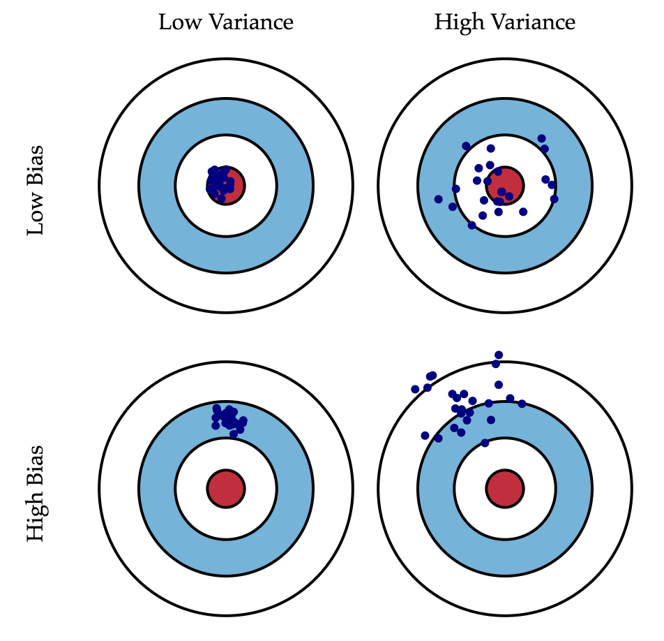
While we cannot do anything with the latter, we can somehow influence the first two. Ideally, we'd like to negate both these terms (upper left square of the picture), but in practice it is often necessary to balance between the biased and unstable estimates (high variance).

Generally, with increasing complexity of the model (e.g., when the number of absolute parameters grows) the variance (dispersion) of the estimate also increases, but bias decreases. Due to the fact that the training set is memorized completely instead of generalising, small changes lead to unexpected results (overfitting). On the other side, if the model is weak it will not be able to learn the pattern, resulting in learning something different that is offset with respect to the right solution.

Gauss-Markov theorem asserts that the OLS estimation of parameters of the linear model is the best in the class of unbiased linear estimates, that is, with the smallest variance. This means that if there exists any other unbiased model $inline$g$inline$, also from class of linear models, we can be sure that $inline$Var\left(\hat{f}\right) \leq Var\left(g\right)$inline$.

Regularization of Linear Regression

Sometimes there are situations when we intentionally increase the bias of the model for the sake of its stability, ie to reduce the variance of the model $inline$\text{Var}\left(\hat{f}\right)$inline$. One of the conditions of Gauss-Markov theorem is a full column rank of matrix $inline$X$inline$. Otherwise OLS solution $inline$\vec{w} = \left(X^T X\right)^{-1} X^T \vec{y}$inline$ does not exist, since the inverse matrix $inline$\left(X^T X\right)^{-1}.$inline$ does not exist. In other words, matrix $inline$X^T X$inline$ will be singular or degenerate. This problem is called ill-posed. The problem must be corrected, namely, matrix $inline$X^T X$inline$ needs to be made non-degenerate, or regular (which is why this process is called regularization). Often we observe in the data the so-called multicollinearity: when two or more features are strongly correlated, it is manifested in the matrix $inline$X$inline$ in the form of "almost" linear dependence between the columns.For example, in the problem of forecasting house price by its parameters, attributes "area with balcony" and "area without balcony" will have such "almost" linear relationship. Formally, matrix $inline$X^T X$inline$ for such data is reversible, but due to multicollinearity some of its eigenvalues will be close to zero, and in the inverse matrix $inline$X^T X$inline$ some extremely large eigenvalues will appear, as eigenvalues ​​of the inverse matrix are $inline$\frac{1}{\lambda_i}$inline$. The result of this vacillation of eigenvalues ​​is unstable estimate of model parameters, ie adding a new set of observations to the training data will lead to a completely different solution. You can find illustration of growth of coefficients in one of our previous posts. One way of regularization is Tikhonov regularization, which generally looks like the addition of a new member to the mean square error:

$$display$$\large \begin{array}{rcl} \mathcal{L}\left(X, \vec{y}, \vec{w} \right) &=& \frac{1}{2n} \left| \vec{y} - X \vec{w} \right|_2^2 + \left|\Gamma \vec{w}\right|^2\ \end{array}$$display$$

Tikhonov matrix is ​​often expressed as the product of a number by the identity matrix: $inline$\Gamma = \frac{\lambda}{2} E$inline$. In this case, the problem of minimization of the mean square error becomes the problem with a restriction on the $inline$L_2$inline$ norm. If we differentiate the new cost function with respect to the model parameters, set the resulting function to zero, and express $inline$\vec{w}$inline$, we get the exact solution of the problem.

$$display$$\large \begin{array}{rcl} \vec{w} &=& \left(X^T X + \lambda E\right)^{-1} X^T \vec{y} \end{array}$$display$$

This regression is called ridge regression. And the ridge is just a diagonal matrix that we add to the $inline$X^T X$inline$ matrix to ensure that we get a regular matrix as a result.

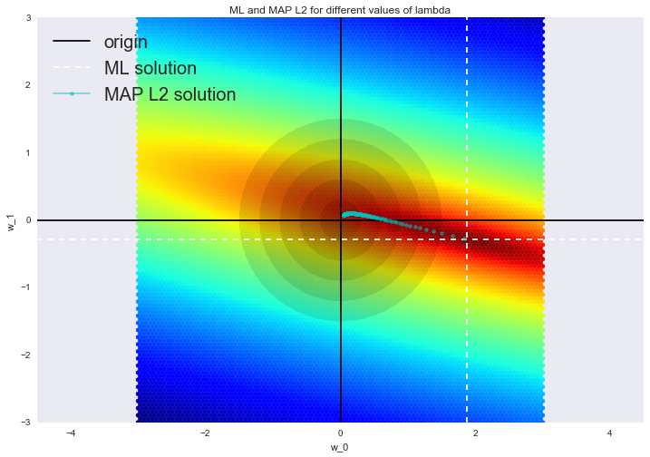
Such a solution reduces the dispersion but becomes biased, because the norm of the vector of parameters is also minimized, which makes the solution to shift towards zero. On the figure below, OLS solution is at the intersection of the white dotted lines. Blue dots represent different solutions of ridge regression. It can be seen that by increasing the regularization parameter $inline$\lambda$inline$, we shift the solution towards zero.

We advise to see our last post for an example of how $inline$L_2$inline$ regularization copes with the problem of multicollinearity, and to refresh the memory of a few interpretations of regularization.

2. Logistic Regression

Linear Classifier

The basic idea of ​​the linear classifier is that the feature space can be divided into two subspaces by a hyperplane, and in each of these subspaces one of two values of the target class is predicted . If this can be done without error, the training set is called linearly separable.

We are already familiar with linear regression and least squares method. Let's consider the binary classification problem, and denote target class tags to be "+1" (positive examples) and "-1" (bad examples). One of the most simple linear classifiers is obtained based on a regression like so:

$$display$$\large a(\vec{x}) = sign(\vec{w}^Tx),$$display$$

where

• $inline$\vec{x}$inline$ is feature vector (along with identity);
• $inline$\vec{w}$inline$ are weights in the linear model (with bias $inline$w_0$inline$);
• $inline$sign(\bullet)$inline$ is a "Signum" function that returns the sign of its argument;
• $inline$a(\vec{x})$inline$ is classifier response for example $inline$\vec{x}$inline$.

Logistic Regression as a Linear Classifier

Logistic regression is a special case of a linear classifier, but it has a good "skill" to predict the probability $inline$p_+$inline$ of referring example $inline$\vec{x_i}$inline$ to the class "+":

$$display$$\large p_+ = P\left(y_i = 1 \mid \vec{x_i}, \vec{w}\right) $$display$$

Prediction of not just a response ( "+1" or "-1"), but the probability of assignment to class "+1" is a very important business requirement in many problems. For example, in the problem of credit scoring where logistic regression is traditionally used, the probability of default ($inline$p_+$inline$) is often predicted. Customers who have applied for a loan are ranked based on this predicted probability (in descending order), and a scoreboard is obtained, which is in fact the customers rating from bad to good. Below is an example of such a toy scoreboard.

The bank chooses a threshold $inline$p_*$inline$ to predict probability of loan default (in the picture it's $inline$0.15$inline$) and starting from this value stops issuing loans. Moreover, it is possible to multiply this predicted probability by outstanding amount and get the expectation of losses from the client, which will also be a good business metrics (further in comments scoring experts can correct me, but the main gist is about this).

So we want to predict the probability $inline$p_+ \in [0,1]$inline$, and now can only construct a linear prediction using OLS: $inline$b(\vec{x}) = \vec{w}^T \vec{x} \in \mathbb{R}$inline$. How to convert the resulting value to the probability that lies in the [0, 1] range? Obviously, this requires some function $inline$f: \mathbb{R} \rightarrow [0,1].$inline$. The logistic regression model takes a specific function for this: $inline$\sigma(z) = \frac{1}{1 + \exp^{-z}}$inline$. Now let's understand what are the prerequisites for this.

Let's denote the probability of event $inline$X$inline$ $inline$P(X)$inline$. Then the ratio of probabilities $inline$OR(X)$inline$ is determined from $inline$\frac{P(X)}{1-P(X)}$inline$, and that is the ratio of probabilities whether or not an event will happen. It is obvious that the probability and odds ratio contain the same information. But while $inline$P(X)$inline$ ranges from 0 to 1, $inline$OR(X)$inline$ is in the range of 0 to $inline$\infty$inline$.

If we calculate the logarithm of the $inline$OR(X)$inline$ (that is called a logarithm of odds, or log probability ratio), it is easy to notice that $inline$\log{OR(X)} \in \mathbb{R}$inline$. This is what we will predict with the OLS.

Let's see how logistic regression will make a prediction $inline$p_+ = P\left(y_i = 1 \mid \vec{x_i}, \vec{w}\right)$inline$ (let's assume for now that we've somehow obtained weights $inline$\vec{w}$inline$ (ie trained the model), later we'll look at how it is done).

• Step 1. Evaluate $inline$w_{0}+w_{1}x_1 + w_{2}x_2 + ... = \vec{w}^T\vec{x}$inline$. (Equation $inline$\vec{w}^T\vec{x} = 0$inline$ defines a hyperplane separating the examples in two classes);

• Step 2. Compute the log odds ratio: $inline$ \log(OR_{+}) = \vec{w}^T\vec{x}$inline$.

• Step 3. Having the forecast of chances to assign an example to the class of "+" - $inline$OR_{+}$inline$, calculate $inline$p_{+}$inline$ calculated using the simple relationship:

$$display$$\large p_{+} = \frac{OR_{+}}{1 + OR_{+}} = \frac{\exp^{\vec{w}^T\vec{x}}}{1 + \exp^{\vec{w}^T\vec{x}}} = \frac{1}{1 + \exp^{-\vec{w}^T\vec{x}}} = \sigma(\vec{w}^T\vec{x})$$display$$

On the right side we have obtained right the sigmoid function.

So, logistic regression predicts the probability of assigning an example to the class of "+" (assuming that we know its characteristics and weights of the model) as a sigmoid transformation of a linear combination of the weight vector and the feature vector:

$$display$$\large p_+(x_i) = P\left(y_i = 1 \mid \vec{x_i}, \vec{w}\right) = \sigma(\vec{w}^T\vec{x_i}). $$display$$

The next question is: how to model is trained? Here again we appeal to the principle of maximum likelihood.

The Principle of Maximum Likelihood and Logistic Regression

Now let's see how an optimization problem for logistic regression is obtained from the principle of maximum likelihood, namely, minimization of the logistic loss function. We have just seen that the logistic regression models the probability of assigning an example to the class of "+" as:

$$display$$\large p_+(\vec{x_i}) = P\left(y_i = 1 \mid \vec{x_i}, \vec{w}\right) = \sigma(\vec{w}^T\vec{x_i})$$display$$

Then for the class "-" similar probability is: $$display$$\large p_-(\vec{x_i}) = P\left(y_i = -1 \mid \vec{x_i}, \vec{w}\right) = 1 - \sigma(\vec{w}^T\vec{x_i}) = \sigma(-\vec{w}^T\vec{x_i}) $$display$$

Both of these expressions can be cleverly combined into one (watch my hands, maybe you are being tricked):

$$display$$\large P\left(y = y_i \mid \vec{x_i}, \vec{w}\right) = \sigma(y_i\vec{w}^T\vec{x_i})$$display$$

Expression $inline$M(\vec{x_i}) = y_i\vec{w}^T\vec{x_i}$inline$ is called margin of classification on the object $inline$\vec{x_i}$inline$ (not to be confused with a gap (also called margin) in the SVM context). If it is non-negative, the model does not make mistake on the object $inline$\vec{x_i}$inline$, if it's negative then class for object $inline$\vec{x_i}$inline$ is misclassified. Note that the margin is defined for objects in the training set only where real target class labels $inline$y_i$inline$ are known.

To understand exactly why we have done such a conclusion, let us turn to the geometrical interpretation of the linear classifier. Details about this can be found in materials by Evgeny Sokolov.

I recommend to solve an almost classical problem from the introductory course of linear algebra: find the distance from the point with a radius-vector $inline$\vec{x_A}$inline$ to a plane which is defined by the equation $inline$\vec{w}^T\vec{x} = 0.$inline$

$$display$$\large \rho(\vec{x_A}, \vec{w}^T\vec{x} = 0) = \frac{\vec{w}^T\vec{x_A}}{||\vec{w}||}$$display$$

When we get (or see) the answer, we will understand that the greater the absolute value of expression $inline$\vec{w}^T\vec{x_i}$inline$, the farther point $inline$\vec{x_i}$inline$ is on the plane $inline$\vec{w}^T\vec{x} = 0.$inline$

Hence, the expression $inline$M(\vec{x_i}) = y_i\vec{w}^T\vec{x_i}$inline$ is a kind of "confidence" of the model in the classification of object $inline$\vec{x_i}$inline$:

• If the margin is large (in absolute value) and positive, it means that the class label is set correctly, and the object is far away from the separating hyperplane (such an object is classified confidently). Point $inline$x_3$inline$ on the picture.
• if the margin is large (in absolute value) and negative, then class label is set incorrectly and the object is far from the separating hyperplane (most likely an object is an anomaly, for example it was improperly labeled in the training set). Point $inline$x_1$inline$ on the picture. if the margin is small (in absolute value), then the object is close to the separating hyperplane and margin sign determines whether the object is correctly classified. Points $inline$x_2$inline$ and $inline$x_4$inline$ on the plot.

Let's now spell out details of the likelihood of the sample, ie the probability of observing the given vector $inline$\vec{y}$inline$ from sample $inline$X$inline$. We'll make a strong assumption: objects come independently from one distribution (i.i.d.).Then

$$display$$\large P\left(\vec{y} \mid X, \vec{w}\right) = \prod_{i=1}^{\ell} P\left(y = y_i \mid \vec{x_i}, \vec{w}\right),$$display$$

where $inline$\ell$inline$ is length of sample $inline$X$inline$ (number of rows).

As usual, let's take the logarithm of this expression (sum is much easier to optimize than the product):

$$display$$\large \begin{array}{rcl} \log P\left(\vec{y} \mid X, \vec{w}\right) &=& \log \prod_{i=1}^{\ell} P\left(y = y_i \mid \vec{x_i}, \vec{w}\right) \ &=& \log \prod_{i=1}^{\ell} \sigma(y_i\vec{w}^T\vec{x_i}) \ &=& \sum_{i=1}^{\ell} \log \sigma(y_i\vec{w}^T\vec{x_i}) \ &=& \sum_{i=1}^{\ell} \log \frac{1}{1 + \exp^{-y_i\vec{w}^T\vec{x_i}}} \ &=& - \sum_{i=1}^{\ell} \log (1 + \exp^{-y_i\vec{w}^T\vec{x_i}}) \end{array}$$display$$

This is, in this case principle of maximization of likelihood leads to minimization of the expression

$$display$$\large \mathcal{L_{log}} (X, \vec{y}, \vec{w}) = \sum_{i=1}^{\ell} \log (1 + \exp^{-y_i\vec{w}^T\vec{x_i}}).$$display$$

This is logistic loss function that is summed over all objects in the training set.

Let's look at the new functions as a function of margin: $inline$L(M) = \log (1 + \exp^{-M})$inline$. Let's plot it along with zero-one loss graph, which simply penalizes the model for errors on each object by 1 (negative margin): $inline$L_{1/0}(M) = [M < 0]$inline$.

The picture reflects the general idea that if we are not able to directly minimize the number of errors in classification problem (at least not by the gradient methods - derivative of 1/0 loss function at zero turns to infinity), we minimize some of its upper bounds. In this case it is logistic loss function (where the logarithm is binary, but it does not matter), and the following is fair:

$$display$$\large \begin{array}{rcl} \mathcal{L_{1/0}} (X, \vec{y}, \vec{w}) &=& \sum_{i=1}^{\ell} [M(\vec{x_i}) < 0] \ &\leq& \sum_{i=1}^{\ell} \log (1 + \exp^{-y_i\vec{w}^T\vec{x_i}}) \ &=& \mathcal{L_{log}} (X, \vec{y}, \vec{w}) \end{array}$$display$$

where $inline$\mathcal{L_{1/0}} (X, \vec{y} is simply the number of errors of logistic regression with weights $inline$\vec{w}$inline$ on a sample $inline$(X, \vec{y})$inline$.

Thus by reducing upper bound $inline$\mathcal{L_{log}}$inline$ by the number of classification errors, we also hope to reduce the number of errors itself.

$inline$L_2$inline$-Regularization of Logistic Loss

L2-regularization of logistic regression is arranged almost the same as the ridge regression. Instead of functional $inline$\mathcal{L_{log}} (X, \vec{y}, \vec{w})$inline$ we minimize the following:

$$display$$\large J(X, \vec{y}, \vec{w}) = \mathcal{L_{log}} (X, \vec{y}, \vec{w}) + \lambda |\vec{w}|^2$$display$$

In the case of logistic regression, reverse regularization coefficient $inline$C = \frac{1}{\lambda}$inline$ is usually introduced. Then the solution of the problem will be:

$$display$$\large \hat{w} = \arg \min_{\vec{w}} J(X, \vec{y}, \vec{w}) = \arg \min_{\vec{w}}\ (C\sum_{i=1}^{\ell} \log (1 + \exp^{-y_i\vec{w}^T\vec{x_i}})+ |\vec{w}|^2)$$display$$

Next, let us consider an example that allows to intuitively understand one of the meanings of regularization.

3. An Illustrative Example of Logistic Regression Regularization

In the first article it has already been shown how the polynomial features allow linear models to build nonlinear separating surfaces. Let's show this in pictures.

Let's see how regularization affects the quality of classification on a dataset on microchip testing from Andrew Ng course on machine learning. We'll use logistic regression with polynomial features and vary regularization parameter C. First, let's see how regularization affects the separating border of the classifier and intuitively recognize under- and overfitting. Then we'll establish regularization parameter to be numerically close to optimal via cross-validation and grid search.

```python from __future__ import division, print_function # turning off Anaconda warnings import warnings warnings.filterwarnings('ignore') %matplotlib inline from matplotlib import pyplot as plt import seaborn as sns

import numpy as np import pandas as pd from sklearn.preprocessing import PolynomialFeatures from sklearn.linear_model import LogisticRegression, LogisticRegressionCV from sklearn.model_selection import cross_val_score, StratifiedKFold from sklearn.model_selection import GridSearchCV

</spoiler>


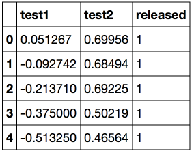
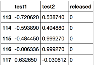
Let's load the data using method read_csv from pandas library. In this dataset on 118 microchips (objects), there are results of two tests for quality control (two numerical variables) and information whether the microchip went into production. Variables are already centered, that is column means are ​​subtracted from all values. Thus, the "average" microchip corresponds to zero values ​​of test results.  

<spoiler title="Loading data">
```python
data = pd.read_csv('../../data/microchip_tests.txt',
header=None, names = ('test1','test2','released'))
# information about dataset
data.info()

<class 'pandas.core.frame.DataFrame'> RangeIndex: 118 entries, 0 to 117 Data columns (total 3 columns): test1 118 non-null float64 test2 118 non-null float64 released 118 non-null int64 dtypes: float64(2), int64(1) memory usage: 2.8 KB

Let's look at the first and last 5 lines.

Let's save the training set and the target class labels in separate NumPy arrays. Let's plot the data. Red corresponds to defective chips, green to normal ones.

```python X = data.ix[:,:2].values y = data.ix[:,2].values ```

plt.scatter(X[y == 1, 0], X[y == 1, 1], c='green', label='Released')
plt.scatter(X[y == 0, 0], X[y == 0, 1], c='red', label='Faulty')
plt.xlabel("Test 1")
plt.ylabel("Test 2")
plt.title('2 tests of microchips')
plt.legend();

Let's define a function to display the separating curve of the classifier

```python def plot_boundary(clf, X, y, grid_step=.01, poly_featurizer=None): x_min, x_max = X[:, 0].min() - .1, X[:, 0].max() + .1 y_min, y_max = X[:, 1].min() - .1, X[:, 1].max() + .1 xx, yy = np.meshgrid(np.arange(x_min, x_max, grid_step), np.arange(y_min, y_max, grid_step))

assign each point in the grid [x_min, m_max]x[y_min, y_max]

its color

Z = clf.predict(poly_featurizer.transform(np.c_[xx.ravel(), yy.ravel()])) Z = Z.reshape(xx.shape) plt.contour(xx, yy, Z, cmap=plt.cm.Paired)

</spoiler>


We call the following polynomial features of degree $inline$d$inline$ for two variables $inline$x_1$inline$ and $inline$x_2$inline$:

$$display$$\large \{x_1^d, x_1^{d-1}x_2, \ldots x_2^d\} =  \{x_1^ix_2^j\}_{i+j=d, i,j \in \mathbb{N}}$$display$$

For example, for $inline$d=3$inline$ this will be the following features:

$$display$$\large 1, x_1, x_2,  x_1^2, x_1x_2, x_2^2, x_1^3, x_1^2x_2, x_1x_2^2, x_2^3$$display$$

If you draw a triangle of Pythagoras, you'll figure out how many of these features there will be for $inline$d=4,5...$inline$ and any other d.
Simply put, the number of such features is exponentially large, and it can be costly to build, say, polynomial features of degree 10 for 100 variables (and more importantly, it's not needed). 


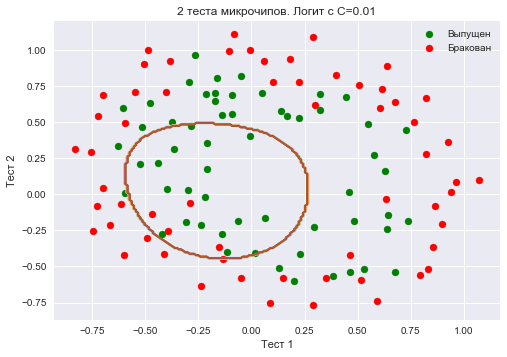
Let's create sklearn object that will add polynomial features up to degree 7 to matrix $inline$X$inline$ and train logistic regression with regularization parameter $inline$C = 10^{-2}$inline$. Let's plot separating border.
We'll also check the proportion of correct answers of the classifier on the training set. We see that regularization was too strong, and the model is underfitted. Percentage of correct answers of the classifier on the training set is 0.627.

<spoiler title="Сщву">
```python
poly = PolynomialFeatures(degree=7)
X_poly = poly.fit_transform(X)

C = 1e-2
logit = LogisticRegression(C=C, n_jobs=-1, random_state=17)
logit.fit(X_poly, y)

plot_boundary(logit, X, y, grid_step=.01, poly_featurizer=poly)

plt.scatter(X[y == 1, 0], X[y == 1, 1], c='green', label='Released')
plt.scatter(X[y == 0, 0], X[y == 0, 1], c='red', label='Faulty')
plt.xlabel("Test 1")
plt.ylabel("Test 2")
plt.title('2 tests of microchips. Logit with C=0.01')
plt.legend();

print("Share of classifier’s correct answers on training set:", 
round(logit.score(X_poly, y), 3))

Let's now increase $inline$C$inline$ to 1. By this we weaken regularization, and now the solution can have greater (in absolute value) values of weights of logistic regression than in the previous case.Now the percentage of correct answers of the classifier on the training set is 0.831.

```python C = 1 logit = LogisticRegression(C=C, n_jobs=-1, random_state=17) logit.fit(X_poly, y)

plot_boundary(logit, X, y, grid_step=.005, poly_featurizer=poly)

plt.scatter(X[y == 1, 0], X[y == 1, 1], c='green', label='Released') plt.scatter(X[y == 0, 0], X[y == 0, 1], c='red', label='Faulty') plt.xlabel("Test 1") plt.ylabel("Test 2") plt.title('2 tests of microchips. Logit with C=1') plt.legend();

print("Share of classifier’s correct answers on training set:", round(logit.score(X_poly, y), 3))

</spoiler>

<img src='https://habrastorage.org/files/f19/876/60a/f1987660a43441a0bc495d89ee141ae4.png' align='center' width=80%><br>


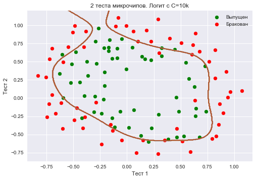
Let's increase $inline$C$inline$ even more - up to 10 thousand. Now regularization is clearly not strong enough, and we see overfitting. Note that in the previous case (with $inline$C$inline$=1 and "smooth" boundary), the share of correct answers on the training set is not much lower than in the third case. But you can easily imagine that on new data the second model will work much better.
Percentage of correct answers of the classifier on the training set is 0.873.


<spoiler title="Code">
```python
C = 1e4
logit = LogisticRegression(C=C, n_jobs=-1, random_state=17)
logit.fit(X_poly, y)

plot_boundary(logit, X, y, grid_step=.005, poly_featurizer=poly)

plt.scatter(X[y == 1, 0], X[y == 1, 1], c='green', label='Released')
plt.scatter(X[y == 0, 0], X[y == 0, 1], c='red', label='Faulty')
plt.xlabel("Test 1")
plt.ylabel("Test 2")
plt.title('2 tests of microchips. Logit with C=10k')
plt.legend();

print("Share of classifier’s correct answers on training set:", 
round(logit.score(X_poly, y), 3))

To discuss the results, let's rewrite functional that is optimized in the logistic regression to the form:

$$display$$\large J(X,y,w) = \mathcal{L} + \frac{1}{C}||w||^2,$$display$$

where

• $inline$\mathcal{L}$inline$ is logistic loss function summed over the entire sample
• $inline$C$inline$ is reverse regularization coefficient (the very same $inline$C$inline$ from sklearn implementation of LogisticRegression)

Interim conclusions:

• the greater the parameter $inline$C$inline$, the more complex relationships in the data model can recover (intuitively $inline$C$inline$ corresponds to the "complexity" of the model (model capacity))
• if regularization is too strong (small values of $inline$C$inline$), the solution of the problem of minimizing the logistic loss function may be the one where many of the weights are zeroed or too small. They also say that the model is not sufficiently "penalized" for errors (ie, in the functional $inline$J$inline$ the sum of the squares of the weights "outweighs", and the error $inline$\mathcal{L}$inline$ can be relatively large). In this case, the model will underfit (first case)
• conversely, if regularization is too weak (high values of $inline$C$inline$), a vector $inline$w$inline$ with high absolute value components can become the solution of the optimization problem. In this case, $inline$\mathcal{L}$inline$ has a greater contribution to the optimized functional $inline$J$inline$, loosely speaking, the model is too "afraid" to be mistaken on the objects from the training set and will therefore overfit (third case)
• logistic regression will not "understand" (or they say "learn") by itself what value of $inline$C$inline$ to choose (in contrast to the weights $inline$w$inline$), that is, it can not be determined by solving the optimization problem that logistic regression is. In the same way, a decision tree can not "understand" by itself what depth limit to choose (not during one learning process). Therefore, $inline$C$inline$ is model's hyperparameter that is tuned on cross-validation, as well as max_depth in a tree.

Tuning the regularization parameter

Now let's find the optimal (for this example) value of the regularization parameter $inline$C$inline$. This can be done via LogisticRegressionCV - grid search of parameters followed by cross-validation. This class is designed specifically for logistic regression (effective algorithms of parameters search are known for it). For an arbitrary model we would use GridSearchCV, RandomizedSearchCV or, for example, special algorithms for hyperparameters optimization implemented in hyperopt.

```python

skf = StratifiedKFold(n_splits=5, shuffle=True, random_state=17)

c_values = np.logspace(-2, 3, 500)

logit_searcher = LogisticRegressionCV(Cs=c_values, cv=skf, verbose=1, n_jobs=-1) logit_searcher.fit(X_poly, y)

</spoiler>

Let's see how the quality of the model (percentage of correct responses on the training and validation sets) varies with the hyperparameter $inline$C$inline$. 

<img src='https://habrastorage.org/files/4d7/288/42a/4d728842ae994eee99e4b1d3329ceaf6.png' align='center' width=80%><br>


Let's select the area with the "best" values of ​​C.

<img src='https://habrastorage.org/files/af9/27c/1cc/af927c1ccd1348928c7b7dba644f118e.png' align='center' width=80%><br>


As we remember, these curves are called *validation* curves, and before we built them manually, but sklearn has special methods for their construction that we too are going to use now.


# 4. Where Logistic Regression Is Good and Where It's Not

### Analysis of IMDB movie reviews

Let's now solve the problem of binary classification of IMDB movie reviews. There is a training set with the marked reviews, for 12500 reviews we know that they are good, for another 12500 we know that they are bad. Here, it's not that easy to get started with machine learning right away because we don't have the matrix $inline$X$inline$, we need to prepare it. We will use the simplest approach - bag of words. With this approach, features of the review will be represented by indicators of the presence of each word from the whole corpus in this review. And the corpus is the set of all user reviews. The idea is illustrated by a picture

<img src="https://habrastorage.org/files/a0a/bb1/2e9/a0abb12e9ed94624ade0b9090d26ad66.png" width=80% align='center'><br>

<spoiler title="Import libraries and load data">
```python
from __future__ import division, print_function
# turning off Anaconda warnings
import warnings
warnings.filterwarnings('ignore')
import numpy as np
import matplotlib.pyplot as plt
%matplotlib inline
import seaborn as sns
import numpy as np
from sklearn.datasets import load_files
from sklearn.feature_extraction.text import CountVectorizer, TfidfTransformer, TfidfVectorizer
from sklearn.linear_model import LogisticRegression
from sklearn.svm import LinearSVC

Загрузим данные отсюда. В обучающей и тестовой выборках по 12500 тысяч хороших и плохих отзывов к фильмам.

reviews_train = load_files("YOUR PATH")
text_train, y_train = reviews_train.data, reviews_train.target

print("Number of documents in training data: %d" % len(text_train))
print(np.bincount(y_train))

# поменяйте путь к файлу
reviews_test = load_files("YOUR PATH")
text_test, y_test = reviews_test.data, reviews_test.target
print("Number of documents in test data: %d" % len(text_test))
print(np.bincount(y_test))

Example of a bad review:

'Words can't describe how bad this movie is. I can't explain it by writing only. You have too see it for yourself to get at grip of how horrible a movie really can be. Not that I recommend you to do that. There are so many clich\xc3\xa9s, mistakes (and all other negative things you can imagine) here that will just make you cry. To start with the technical first, there are a LOT of mistakes regarding the airplane. I won't list them here, but just mention the coloring of the plane. They didn't even manage to show an airliner in the colors of a fictional airline, but instead used a 747 painted in the original Boeing livery. Very bad. The plot is stupid and has been done many times before, only much, much better. There are so many ridiculous moments here that i lost count of it really early. Also, I was on the bad guys' side all the time in the movie, because the good guys were so stupid. "Executive Decision" should without a doubt be you're choice over this one, even the "Turbulence"-movies are better. In fact, every other movie in the world is better than this one.'

Example of a good review:

'Everyone plays their part pretty well in this "little nice movie". Belushi gets the chance to live part of his life differently, but ends up realizing that what he had was going to be just as good or maybe even better. The movie shows us that we ought to take advantage of the opportunities we have, not the ones we do not or cannot have. If U can get this movie on video for around $10, it\xc2\xb4d be an investment!'

A Simple Count of Words

Let's compiled a dictionary of all the words with CountVectorizer. The sample contains 74,849 unique words. If you look at the examples of received "words" (let's call them tokens), you can see that we've omitted many of the important steps of text processing (automatic text processing could be the subject of a separate series of articles).

```python cv = CountVectorizer() cv.fit(text_train)

print(len(cv.vocabulary_)) #74849

```python
print(cv.get_feature_names()[:50])
print(cv.get_feature_names()[50000:50050])

['00', '000', '0000000000001', '00001', '00015', '000s', '001', '003830', '006', '007', '0079', '0080', '0083', '0093638', '00am', '00pm', '00s', '01', '01pm', '02', '020410', '029', '03', '04', '041', '05', '050', '06', '06th', '07', '08', '087', '089', '08th', '09', '0f', '0ne', '0r', '0s', '10', '100', '1000', '1000000', '10000000000000', '1000lb', '1000s', '1001', '100b', '100k', '100m'] ['pincher', 'pinchers', 'pinches', 'pinching', 'pinchot', 'pinciotti', 'pine', 'pineal', 'pineapple', 'pineapples', 'pines', 'pinet', 'pinetrees', 'pineyro', 'pinfall', 'pinfold', 'ping', 'pingo', 'pinhead', 'pinheads', 'pinho', 'pining', 'pinjar', 'pink', 'pinkerton', 'pinkett', 'pinkie', 'pinkins', 'pinkish', 'pinko', 'pinks', 'pinku', 'pinkus', 'pinky', 'pinnacle', 'pinnacles', 'pinned', 'pinning', 'pinnings', 'pinnochio', 'pinnocioesque', 'pino', 'pinocchio', 'pinochet', 'pinochets', 'pinoy', 'pinpoint', 'pinpoints', 'pins', 'pinsent']

Let's encode the sentences from the training set texts with indexes if incoming words. We'll use the sparse format. Let's transform the test set in the same way.

X_train = cv.transform(text_train)
X_test = cv.transform(text_test)

Let's train logistic regression and look at the proportion of correct answers on the training and test sets. It turns out that we correctly guess the tone of the review on approximately 86.7% of test cases.

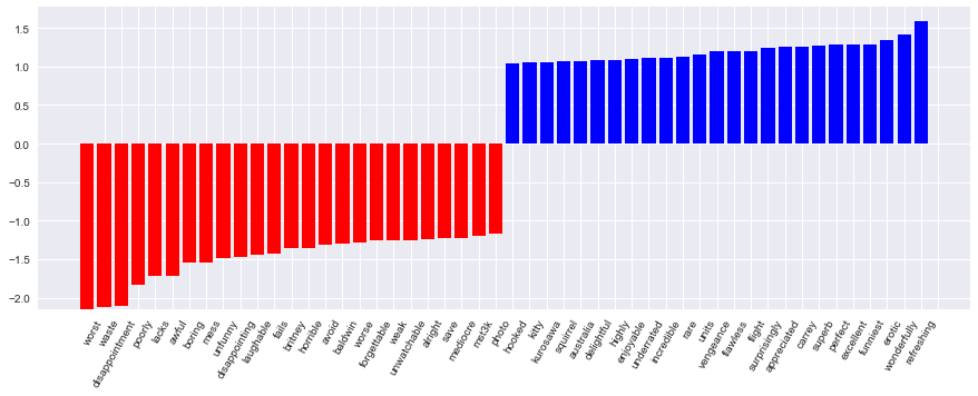
```python %%time logit = LogisticRegression(n_jobs=-1, random_state=7) logit.fit(X_train, y_train) print(round(logit.score(X_train, y_train), 3), round(logit.score(X_test, y_test), 3)) ```

The coefficients of the model can be beautifully displayed.

```python def visualize_coefficients(classifier, feature_names, n_top_features=25): # get coefficients with large absolute values coef = classifier.coef_.ravel() positive_coefficients = np.argsort(coef)[-n_top_features:] negative_coefficients = np.argsort(coef)[:n_top_features] interesting_coefficients = np.hstack([negative_coefficients, positive_coefficients]) # plot them plt.figure(figsize=(15, 5)) colors = ["red" if c < 0 else "blue" for c in coef[interesting_coefficients]] plt.bar(np.arange(2 * n_top_features), coef[interesting_coefficients], color=colors) feature_names = np.array(feature_names) plt.xticks(np.arange(1, 1 + 2 * n_top_features), feature_names[interesting_coefficients], rotation=60, ha="right");

```python
def plot_grid_scores(grid, param_name):
plt.plot(grid.param_grid[param_name], grid.cv_results_['mean_train_score'],
color='green', label='train')
plt.plot(grid.param_grid[param_name], grid.cv_results_['mean_test_score'],
color='red', label='test')
plt.legend();

visualize_coefficients(logit, cv.get_feature_names())

Let's choose the regularization coefficient for the logistic regression. We'll use sklearn.pipeline because CountVectorizer should only be applied to the data that is currently used in training (in order to not "peek" into the test set and not count word frequencies there). In this case, pipeline determines the sequence of actions: apply CountVectorizer, then train logistic regression. So we raise the proportion of correct answers to 88.5% on cross-validation, and to 87.9% on the hold-out set.

```python from sklearn.pipeline import make_pipeline

text_pipe_logit = make_pipeline(CountVectorizer(), LogisticRegression(n_jobs=-1, random_state=7))

text_pipe_logit.fit(text_train, y_train) print(text_pipe_logit.score(text_test, y_test))

from sklearn.model_selection import GridSearchCV

param_grid_logit = {'logisticregression__C': np.logspace(-5, 0, 6)} grid_logit = GridSearchCV(text_pipe_logit, param_grid_logit, cv=3, n_jobs=-1)

grid_logit.fit(text_train, y_train) grid_logit.best_params_, grid_logit.best_score_ plot_grid_scores(grid_logit, 'logisticregression__C') grid_logit.score(text_test, y_test)

</spoiler>


<img src='https://habrastorage.org/files/715/7a4/1ff/7157a41fffc344dabd32ebc65c00ce73.png'><br>



Now let's do the same, but with random forest. We see that with logistic regression we reach a greater proportion of correct answers with less effort. Random Forest works longer and gives 85.5% of correct answers on a hold-out set. 
<spoiler title="Code for training random forest">
```python
from sklearn.ensemble import RandomForestClassifier
forest = RandomForestClassifier(n_estimators=200, n_jobs=-1, random_state=17)
forest.fit(X_train, y_train)
print(round(forest.score(X_test, y_test), 3))

XOR-Problem

Let's now consider an example where linear models work worse.

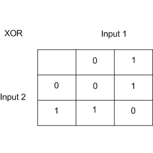
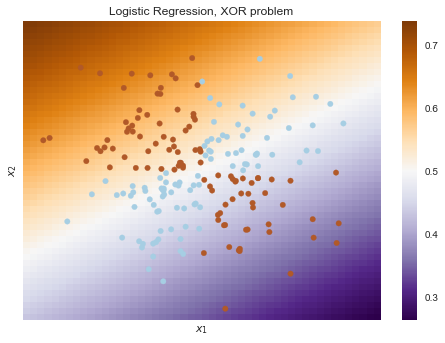
Linear classification methods still build a very simple separating surface - a hyperplane. The most famous toy example of the problem where classes can not be divided by a hyperplane (or line in 2D) with no errors is known as "the XOR problem".

XOR is the "exclusive OR", a Boolean function with the following truth table:

XOR gave the name to a simple binary classification problem, in which the classes are presented as diagonally extended intersecting point clouds.

```python # порождаем данные rng = np.random.RandomState(0) X = rng.randn(200, 2) y = np.logical_xor(X[:, 0] > 0, X[:, 1] > 0) ```

plt.scatter(X[:, 0], X[:, 1], s=30, c=y, cmap=plt.cm.Paired);

def plot_boundary(clf, X, y, plot_title):
xx, yy = np.meshgrid(np.linspace(-3, 3, 50),
np.linspace(-3, 3, 50))
clf.fit(X, y)
# plot the decision function for each datapoint on the grid
Z = clf.predict_proba(np.vstack((xx.ravel(), yy.ravel())).T)[:, 1]
Z = Z.reshape(xx.shape)

image = plt.imshow(Z, interpolation='nearest',
extent=(xx.min(), xx.max(), yy.min(), yy.max()),
aspect='auto', origin='lower', cmap=plt.cm.PuOr_r)
contours = plt.contour(xx, yy, Z, levels=[0], linewidths=2,
linetypes='--')
plt.scatter(X[:, 0], X[:, 1], s=30, c=y, cmap=plt.cm.Paired)
plt.xticks(())
plt.yticks(())
plt.xlabel(r'$inline$x_1$inline$')
plt.ylabel(r'$inline$x_2$inline$')
plt.axis([-3, 3, -3, 3])
plt.colorbar(image)
plt.title(plot_title, fontsize=12);

plot_boundary(LogisticRegression(), X, y,
"Logistic Regression, XOR problem")

from sklearn.preprocessing import PolynomialFeatures
from sklearn.pipeline import Pipeline

logit_pipe = Pipeline([('poly', PolynomialFeatures(degree=2)), 
('logit', LogisticRegression())])

plot_boundary(logit_pipe, X, y,
"Logistic Regression + quadratic features. XOR problem")

Obviously, one can not draw a straight line so as to separate one class from another without errors. Therefore, logistic regression copes badly with this task.

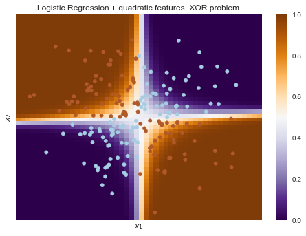
But if you give polynomial features as an input, in this case up to 2 degrees, then the problem is solved.

Here, logistic regression still built a hyperplane, but in a 6-dimensional feature space $inline$1, x_1, x_2, x_1^2, x_1x_2$inline$ and $inline$x_2^2$inline$. In the projection to the original feature space $inline$x_1, x_2$inline$ the boundary is nonlinear.

In practice, polynomial features do help, but it is computationally inefficient to build them explicitly. SVM with kernel trick works much faster. In this approach, only distance between the objects (defined by the kernel function) in a high dimensional space is computed, and there's no need to explicitly produce a combinatorially large number of features. You can read about it in detail in the course of Evgeny Sokolov (contains serious mathematics).

5. Validation and Learning Curves

We've already got an idea of ​​model validation, cross-validation and regularization. Now let's consider the main question:

What to do if the quality of the model is dissatisfying?

• Make the model more complicated or simple?
• Add more features?
• Or we simply need more data for training?

The answers to these questions do not always lie on the surface. In particular, sometimes using a more complex model would lead to a deterioration in performance. Or adding new observations will not lead to noticeable changes. The ability to make the right decision and choose the right way to improve the model, in fact, distinguishes the good professional from the bad one.

We will work with the familiar data on customer churn of telecom operator.

```python from __future__ import division, print_function # turning off Anaconda warnings import warnings warnings.filterwarnings('ignore') %matplotlib inline from matplotlib import pyplot as plt import seaborn as sns

import numpy as np import pandas as pd from sklearn.preprocessing import PolynomialFeatures from sklearn.pipeline import Pipeline from sklearn.preprocessing import StandardScaler from sklearn.linear_model import LogisticRegression, LogisticRegressionCV, SGDClassifier from sklearn.model_selection import validation_curve

data = pd.read_csv('../../data/telecom_churn.csv').drop('State', axis=1) data['International plan'] = data['International plan'].map({'Yes': 1, 'No': 0}) data['Voice mail plan'] = data['Voice mail plan'].map({'Yes': 1, 'No': 0})

y = data['Churn'].astype('int').values X = data.drop('Churn', axis=1).values

</spoiler>


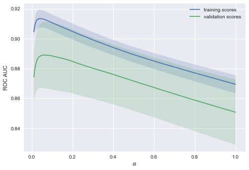
We'll train logistic regression with a stochastic gradient descent. For now we'll just say that it's faster this way, but later in the course we'll have a separate article on this matter. Let's construct validation curves showing how the quality (ROC AUC) on train and test sets varies with the regularization parameter.

<spoiler title="Code">
```python
alphas = np.logspace(-2, 0, 20)
sgd_logit = SGDClassifier(loss='log', n_jobs=-1, random_state=17)
logit_pipe = Pipeline([('scaler', StandardScaler()), ('poly', PolynomialFeatures(degree=2)), 
('sgd_logit', sgd_logit)])
val_train, val_test = validation_curve(logit_pipe, X, y,
'sgd_logit__alpha', alphas, cv=5,
scoring='roc_auc')

def plot_with_err(x, data, **kwargs):
mu, std = data.mean(1), data.std(1)
lines = plt.plot(x, mu, '-', **kwargs)
plt.fill_between(x, mu - std, mu + std, edgecolor='none',
facecolor=lines[0].get_color(), alpha=0.2)

plot_with_err(alphas, val_train, label='training scores')
plot_with_err(alphas, val_test, label='validation scores')
plt.xlabel(r'$\alpha$'); plt.ylabel('ROC AUC')
plt.legend();

The trend is visible at once, and it is very common.

• For simple models, training and validation errors are somewhere nearby, and they are large.This suggests that the model is underfitted, that is, it doesn't have a sufficient number of parameters.

• For highly sophisticated models training and validation errors differ significantly.This can be explained by overfitting: when there are too many parameters or regularization is not strict enough, algorithm can be "distracted" by the noise in the data and lose the major trend.

How much data is needed?

It is known that the more data the model uses the better. But how do we understand in a given situation whether new data will help or not? For example, is it rational to spend N$ for assessors work to double the dataset?

Since the new data can be not available, it is reasonable to vary the size of the training set and see how the quality of the solution depends on the amount of data on which we trained model. This is how we get the learning curves.

The idea is simple: we display the error as a function of the number of examples used for training. The parameters of the model are fixed in advance.

Let's see what we get for the linear model. Let's set the regularization coefficient quite large.

```python from sklearn.model_selection import learning_curve

def plot_learning_curve(degree=2, alpha=0.01): train_sizes = np.linspace(0.05, 1, 20) logit_pipe = Pipeline([('scaler', StandardScaler()), ('poly', PolynomialFeatures(degree=degree)), ('sgd_logit', SGDClassifier(n_jobs=-1, random_state=17, alpha=alpha))]) N_train, val_train, val_test = learning_curve(logit_pipe, X, y, train_sizes=train_sizes, cv=5, scoring='roc_auc') plot_with_err(N_train, val_train, label='training scores') plot_with_err(N_train, val_test, label='validation scores') plt.xlabel('Training Set Size'); plt.ylabel('AUC') plt.legend()

plot_learning_curve(degree=2, alpha=10)

</spoiler>

<img src='https://habrastorage.org/files/ccd/d66/8ec/ccdd668ec5d042ca8cefc0e91681fedb.png' align='center' width=80%><br>


A typical situation: for a small amount of data errors on training and cross-validation sets are quite different, indicating overfitting. For the same model, but with a large amount of data errors "converge" which indicates underfitting.
 
If we add more data, error on the training set will not grow, but on the other hand, the error on the test data will not be reduced.
 
So the errors "converged" and the addition of new data will not help. Actually this case is the most interesting for business. It is possible that we increase the dataset 10 times. But if you do not change the complexity of the model, it may not help. That is the strategy "set once, then use 10 times" might not work.
 
What happens if we change the regularization coefficient (reduce to 0.05)?
 
We see a good trend - the curves gradually converge, and if we move farther to the right (add more data to the model), we can improve the quality on the validation even more. 


<img src='https://habrastorage.org/files/111/631/1aa/1116311aaf2848db9c5ef4d4c6f993b3.png' align='center' width=80%><br>


And what if we make the model even more complex (alpha = 10-4)?

Overfitting is seen - AUC decreases both on training, and on validation sets.

<img src='https://habrastorage.org/files/f65/b03/f62/f65b03f62a6f47de9e70b53691798b5c.png' align='center' width=80%><br>


Constructing these curves can help to understand which way to go and how to properly adjust the complexity of the model on new data.

**Conclusions on the learning and validation curves**

- Error on the training set says nothing about the quality of the model by itself
- Cross-validation error shows how well the model fits the data (the existing trend in the data), while retaining the ability to generalize to new data
- **Validation curve** is a graph showing the result on training and validation sets depending on the **complexity of the model**:
+ if the two curves are close to each other and both errors are large, it's a sign of *underfitting*
+ If the two curves are far from each other, it's a sign of *overfitting*
- **Learning Curve** is a graph showing the results on validation and training sets depending on the number of observations:
+ if the curves converged to each other, adding new data won't help and it is necessary to change the complexity of the model 
+ if the curves haven't converged, adding new data can improve the result.


# 6. Pros and Cons of Linear Models in Machine Learning Problems 

Pros:
- Well studied
- Very fast, can run on very large datasets
- Hands-down winners when there are very many features (hundreds of thousands or more) and they are sparse (although there also exist factorization machines)
- The coefficients of the features can be interpreted (provided that the features are scaled) - in linear regression, as partial derivatives of the features with respect to the target variable, in logistic regression - as a change of chances of referring to one or another class by $inline$\exp^{\beta_i}$inline$ times while feature $inline$x_i$inline$ changes by 1, more [here](https://www.unm.edu/~schrader/biostat/bio2/Spr06/lec11.pdf)
- Logistic regression outputs the probability of assignment to different classes (this is very much appreciated, for example, in credit scoring)
- The model can build nonlinear boundaries given the polynomial features as an input

Cons:
- Perform poorly in tasks where the dependence of the responses from the features is complex, nonlinear
- In practice, the assumptions of Gauss-Markov theorem are almost never fulfilled, so often linear methods perform worse than, for example, SVM and ensembles (judging by the quality classification/regression)

# 7. Homework #4
This time homework is large and consists of two parts – [part 1](https://github.com/Yorko/mlcourse_open/tree/master/jupyter_notebooks/topic4_linear_models/hw4_part1_websites_logistic_regression.ipynb) and [part 2](https://github.com/Yorko/mlcourse_open/tree/master/jupyter_notebooks/topic4_linear_models/hw4_part2_habr_popularity_ridge.ipynb). You need to repeat basic solutions of two Kaggle Inclass competitions by following instructions.

Ответы надо заполнить в [веб-форме](https://goo.gl/forms/xA3xkNkgMp1aNdgn2). Максимум за задание – 18 баллов. Дедлайн – 27 марта 23:59 UTC+3.

**Kaggle Inclass competitions in our course**

Теперь официально представляем 2 соревнования, результаты которых будут учитываться в рейтинге нашего курса:
We now officially present 2 competitions results of which will be considered in the rating of our course: 

- [First](https://inclass.kaggle.com/c/howpop-habrahabr-favs-lognorm) "Predicting article’s popularity"
- [Second](https://inclass.kaggle.com/c/catch-me-if-you-can-intruder-detection-through-webpage-session-tracking) "Identifying hacker by sequence of websites visited". 

Details about the task can be found on the relevant pages of the competition.
For each of the competitions you can receive up to 40 points. The formula for calculating the number of points: $inline$40 (1 - (p-1)/ N)$inline$, where $inline$p$inline$ is the place of the participant in a private ranking, $inline$N$inline$ is number of participants who overcame all benchmarks in a private ranking (new benchmarks may be added) and whose solution satisfies the rules of the competition. Competitions are open throughout the course. 

# 8. Useful resources

- A thorough review of the classics of machine learning and, of course, linear models is made in the "Deep Learning" [book](https://www.deeplearningbook.org/) (I. Goodfellow, Y. Bengio, A. Courville, 2016);
- Implementation of many machine learning algorithms from scratch – [repository](https://github.com/rushter/MLAlgorithms) @rushter. We recommend to take a look at implementation of logistic regression;
- [Курс](https://github.com/esokolov/ml-course-hse) Евгения Соколова по машинному обучению (материалы на GitHub). Хорошая теория, нужна неплохая математическая подготовка;
- [Курс](https://github.com/diefimov/MTH594_MachineLearning) Дмитрия Ефимова на GitHub (англ.). Тоже очень качественные материалы.

*Статья написана в соавторстве с @mephistopheies (Павлом Нестеровым). Авторы домашнего задания – @aiho (Ольга Дайховская) и @das19 (Юрий Исаков). Благодарю @bauchgefuehl (Анастасию Манохину) за редактирование.*