formable provides tools for formability analysis in materials science.

Installation

pip install formable

To support showing visualisations within a Jupyter notebook, you will also need to make sure Plotly is set up to work within the notebook environment:

pip install "notebook>=5.3" "ipywidgets>=7.2"

Getting Started

LoadResponse and LoadResponseSet

The response of a material to a load is represented by the LoadResponse class. Use the following code snippet create a LoadResponse, where the arguments passed represent incremental data (i.e. data for each of the "steps" in the loading):

from formable import LoadResponse

load_response = LoadResponse(true_stress=true_stress, equivalent_strain=equivalent_strain)

true_stress and equivalent_strain are Numpy arrays of shapes (N, 3, 3) and (N,), respectively, for N increments within the load response.

A collection of load responses that contain the same incremental data are represented by the LoadResponseSet class:

from formable import LoadResponse, LoadResponseSet

all_responses = [LoadResponse(...), LoadResponse(...), ...]
load_set = LoadResponseSet(all_responses)

Yield functions

A number of yield functions as defined in the literature can be fitted and visualised. As an example, let's visualise the difference between the Von Mises and the Tresca yield criteria:

from formable.yielding.yield_functions import YieldFunction, VonMises, Tresca

von_mises = VonMises(equivalent_stress=70e6)
tresca = Tresca(equivalent_stress=70e6)

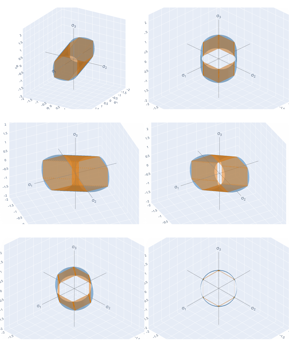
YieldFunction.compare_3D([von_mises, tresca])

If run within a Jupyter environment, this code snippet will generated a 3D visualisation of the yield surfaces in principal stress space:

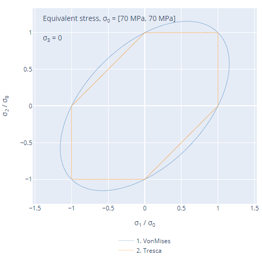
To look at a single plane within principal stress space, we can do this:

YieldFunction.compare_2D([von_mises, tresca], plane=[0, 0, 1])

which generates a figure like this:

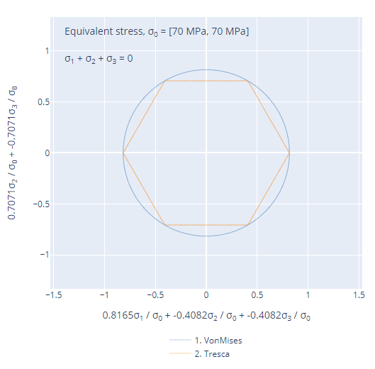
We can choose any plane that intercepts the origin. For instance, we can also look at the π-plane (σ₁ = σ₂ = σ₃):

YieldFunction.compare_2D([von_mises, tresca], plane=[1, 1, 1])

which generates a figure like this:

Yield function fitting

Using experimental or simulated yielding tests, we can fit yield functions to the results. Consider a LoadResponseSet object that has a sufficiently large number of increments of true_stress and equivalent_strain data to enable such a fit. Using the Barlat "Yld2000-2D" anisotropic yield function as an example, we can perform a fit:

from formable import LoadResponse, LoadResponseSet
from formable.yielding import YieldPointCriteria

# First generate a LoadResponseSet, using the results from experiment/simulation:
all_responses = [LoadResponse(...), LoadResponse(...), ...]
load_set = LoadResponseSet(all_responses)

# Then define a yield point criterion:
yield_point = YieldPointCriteria('equivalent_strain', 1e-3)

# Now calculate yield stresses according to the yield point criteria:
load_set.calculate_yield_stresses(yield_point)

# Now we can fit to the resulting yield stresses:
load_set.fit_yield_function('Barlat_Yld2000_2D', equivalent_stress=70e6)

Choosing the fitting parameters and initial guesses

We can specify which of the yield function parameters we would like to fit, and which should remain fixed. We can also pass initial values to the fitting procedure. A least squares fit is employed to fit yield functions in formable.

To fix a parameter during the fit, just pass it as a keyword argument to the fit_yield_function method, as we did in the above example, where we fixed the equivalent_stress parameter. To pass initial values for some of the parameters, we can pass a initial_params dictionary:

load_set.fit_yield_function('Barlat_Yld2000_2D', initial_params={'a1': 1.4})

We can see the available parameters of a given yield function by using the PARAMETERS attribute of a YieldFunction class:

from formable.yielding.yield_functions import Barlat_Yld2000_2D

print(Barlat_Yld2000_2D.PARAMETERS)

which prints:

['a1',
 'a2',
 'a3',
 'a4',
 'a5',
 'a6',
 'a7',
 'a8',
 'equivalent_stress',
 'exponent']

Alternatively, if we have created a yield function object (from a fitting procedure, or directly), we can use the get_parameters method to get the parameters and their values:

print(von_mises.get_parameters())

which prints:

{'equivalent_stress': 70000000.0}

Visualising the fit

Once a yield function has been fit to a load set, we can visualise the fitted yield function like this:

load_set.show_yield_functions_3D()

or, in a similar way to above, we can visualise the fitted yield functions in a given principal stress plane, using:

load_set.show_yield_functions_2D(plane=[0, 0, 1])