SIMBA🦁 workflow description

This article will explain in detail how the pipeline is structured and what are the rationales behind it.

Overview

Basic description

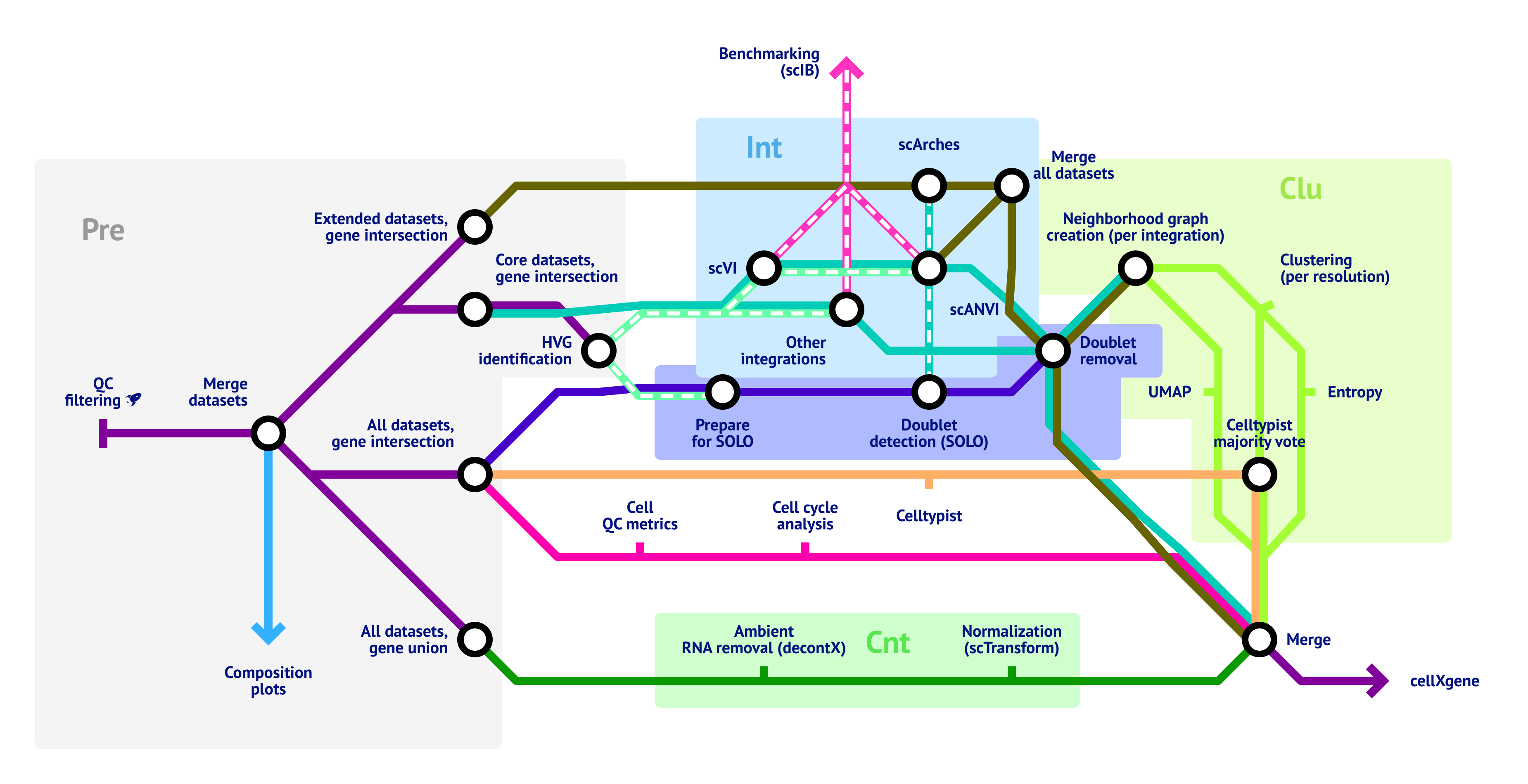
The pipeline can roughly be structured in 6 sections:

• Preprocessing
• Integration
• Clustering
• Doublet detection
• Metadata generation
• Count treatment

These sections will be described in detail below.

Some general technical information

In all of theses sections (except count treatment), pickle files will be created, containing only new information that is generated in each of the tasks. This prevents high storage usage that would occur if each task would save a full copy of the dataset (which can be tens to hundreds of gigabytes large). These incremental pickle files are collected in two nextflow channels: One called obs (one-dimensional data: Clustering, QC metrics) and one called obsm (multi-dimensional data: UMAP, embeddings). The entries of these channels will then be aggregated onto the h5ad file which is generated within the counts section.

Preprocessing

QC of single cell datasets is a very sensitive task and can hardly be automated as part of a pipeline. Thus, we expect users to either filter the input data manually before using SIMBA🦁 or to provide cut-off values via the samplesheet.

Per-dataset preprocessing

During this process, the following things will be checked:

• Does the dataset really contain raw counts?
• Does the dataset contain celly?
• Are all required metadata fields available?
• Are there any duplicates in barcodes or gene names?
• If the no_symbols flag is not set for this dataset, are there exclusively gene symbols in the var_names? If there are any problems found in the checks above, the task terminates and the pipeline proceeds with the "Problem handling" section.

If everything is correct, unnecessary obs columns will be removed, the obs_names will be prefixed with the dataset id and the count matrix will be converted to the CSR sparse format, which helps decreasing the resource usage of the pipeline. Next, gene IDs will be converted to gene symbols using the mygene package if the no_symbols flag is set for this dataset. Afterwards, gene symbols will be converted to uppercase representations and underlines and dots will be converted to dashes, in order to make minimize the probability of having synonym symbols in different datasets. If there are any duplicates in the var_names now, they will be aggregated by calculating the mean. Lastly, cell filtering is performed, if any cut-off values have been provided in the samplesheet.

Problem handling

If there are problems during the per-dataset preprocessing, the pipeline will not fail straightaway. Instead, the pipeline will wait until all datasets have been checked, then write the found problems into a single file and provide it to the user in the run output directory. Once everything is in place, the pipeline will terminate with an error. This makes handling of problems in the input data as convenient as possible.

Merge datasets

This will only be executed if no problems have occured during per-dataset preprocessing. Basically the purpose of this process is to concatenate all datasets into a single annData file. However, it is a little bit more complicated than this.

First, the datasets will be concatenated in two ways:

1. Concatenation of all cells with inner join (intersection) of genes -> integration
2. Concatenation of all cells with outer join (union) of genes -> counts

We are dealing with two constraints here: Biologists want to have as many genes as possible available in order to make good annotations and integration methods require robust data in order to work well. In an optimal world, we now would fill all the missing genes for each datasets with NaN values and both biologists and integration methods would be happy. However, there is a major problem with this: Sparse matrices can only store 0 values implicitly (without using memory), while NaN values use memory. And even though a single NaN does not use a lot of memory, considering that we are dealing with potentially millions of cells, the memory usage would quickly skyrocket. So the solution we came up with is to provide the integration method only with expression values which are available in all datasets while filling up the matrices with 0 values for the "counts" branch of the pipeline. This means that in the final dataset, real 0 values can not be distinguished from artificial 0 values, which needs to be taken into account when analyzing the final output.

Second, all genes that are not expressed in at least one cell of the core datasets will be removed. Additionally, all cells without a single expressed genes will be removed. The purpose of these filters is to prevent zero divisions later on in the pipeline.