Cartpole Simulator

Tutorial

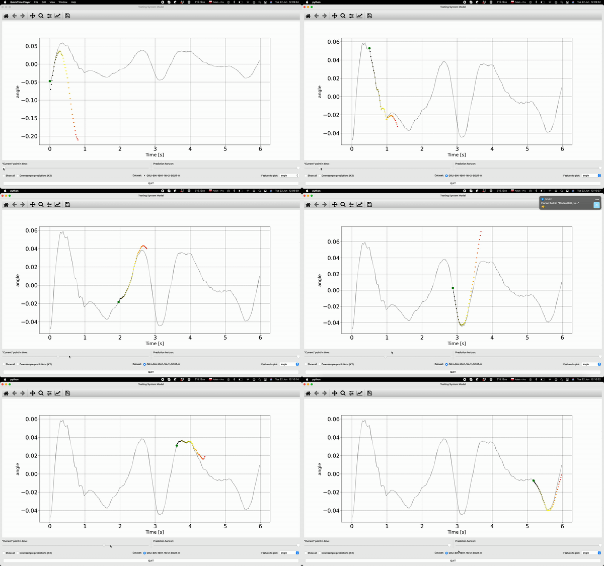
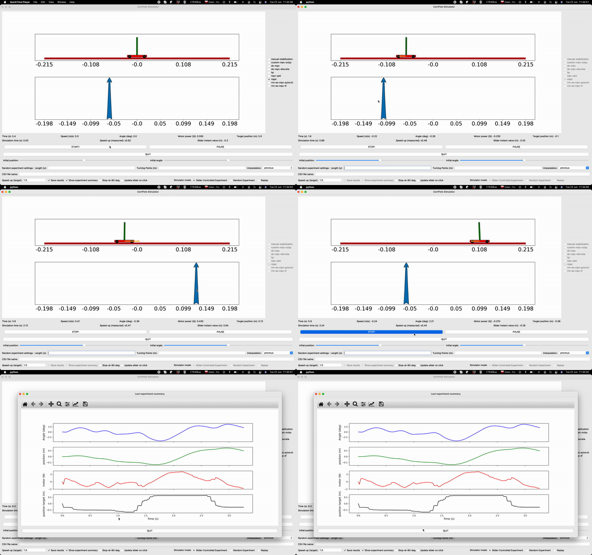
Check our tutorial which will guide you through installation and explain basic functionalities!

A lengthy explanation of the code is provided in this video series.

Installation

Get the code from Github:

git clone --recurse-submodules https://github.com/SensorsINI/CartPoleSimulation.git

Create conda environment with

conda create -n CartPoleSimulation python=3.8
conda activate CartPoleSimulation

If SI_Toolkit (System Identification Toolbox) or Control Toolkit folders are empty, use these lines to pull all submodules:

git submodule update --init --recursive
git submodule update --recursive --remote

Preferable way to install python packages: pip install -r requirements.txt in a conda env or pip venv.

This file was created and tested on macOS, running on Linux and Windows may require some minor changes and/or installing some packages manually. However, the Simulator should work on all major OSes (macOS, Linux, Windows).

Note that you might want to uninstall the ptvsd package unless you use VS Code. This package enables debugging in VS Code, however causes proliferation of useless warnings if imported in another environment.

We created the requirements.txt on macOS with pip list --format=freeze > requirements.txt. It required some minor manual corrections (deleting the package versions) to make the re-installation smooth. It should be also possible to create this file with conda list -e > requirements.txt.

Basic Operation

1. Run GUI: Run python run_cartpole_gui.py from top-level path.
2. Run a single experiment: Open run_data_generator.py. In the marked section, you can define your experiment. For a single run, set number_of_experiments = 1. Then open ./config.yml to modify controller-related parameters. For example, you can choose there whether MPPI should run with the true model ('predictor_ODE_v0' == Euler Integrator) or with a neural network ('predictor_autoregressive_neural'). Once set, run python -m run_data_generator. It will create a new folder ./Experiment_Recordings/ and store a csv log file in it.

Run a Machine Learning Pipeline

You can use this repository to generate training data, train a neural network model using SI_Toolkit, and run the resulting controller.

1. Define all the parameters in config_data_gen.yml to your liking.
2. Run python -m SI_Toolkit_ASF.run.run_data_generator_for_ML_Pipeline. This will create a new experiment folder ./SI_Toolkit_ASF/Experiments/Experiment-[X]/. You will work in this folder from now on. Within there, in Recordings/ there is now a set of CSVs saved and split up into Train/Validate/Test folders. Also, copies of the current configuration files are saved there.
3. In ./SI_Toolkit_ASF/config_training.yml you can now set paths/path_to_experiment: to the newly created one. All pipeline-related scripts access this parameter to know which data to work on and where to store the models.
4. Normalize the data using python -m SI_Toolkit_ASF.run.Create_normalization_file. This creates a normalization file within the experiment folder set in step 3.
5. Train a model using either TensorFlow (default) or PyTorch. Specify the library to use in ./SI_Toolkit_ASF/config_training.yml. Type python -m SI_Toolkit_ASF.run.Train_Network -h for a list of parameters you can define. Some default values are set in the same config as in step 3 and can also be modified there. Now run the Train module with all parameter flags that you wish. You will want to specify the network architecture. Training will store a new model within a subfolder Models/ in the chosen experiment folder.
6. Test the model. Adjust the parameters in ./SI_Toolkit_ASF/config_testing.yml to select the correct test file and model. Run python -m SI_Toolkit_ASF.run.Run_Brunton_Test which selects the test run set in config and compares the model's predictions versus true model behavior in Brunton-style plots. You can again see all params with the flag -h. If the script breaks, set a smaller --test_len.
7. Run MPPI with the trained model. Define an experiment in run_data_generator.py, select "predictor_autoregressive_neural" in the top-level config file, and run python -m run_data_generator. The results can be replayed in GUI.

Structure:

The CartPole class in CartPole folder corresponds to a physical cartpole. It contains methods for setting cartpole parameters, calculating dynamical equation, drawing cartpole and many more.

To perform an experiment CartPole needs an "environment". This environment is provided with CartPole GUI - suitable to visualize dynamical evolution and impact of parameter change - and Data Generator, with which user can easily generate hours of experimental data. They can be started by running run_cartpole_gui.py and run_data_generator.py respectively.

The CartPole loads controllers from Controllers folder. One can specify in GUI or in Data Generator which controller should be used. Adding controllers is easy: They just have to fit the template provided in Control_Toolkit/Controllers/template_controller.py. CartPole-specific controllers can be defined in Control_Toolkit_ASF/Controllers If a file in Controllers folder is named controller_....py and contains the function with the same name (controller_...) it will be automatically detected and added to the list of possible controllers. The MPC controller can be used in combination with any of the optimizers in Control_Toolkit/Optimizers. You can define new optimizers as well

Operation hints:

While the documentation of parameters is still missing in Readme, they are extensively commented in CartPole/cartpole_model.py, GUI/gui_default_params.py and run_data_generator.py. Look inside for more details.

In the “Manual Stabilization” mode you can provide the control input (motor power related to the force acting on the cart) by hovering/clicking with your mouse over the lower chart. Due current Cart-Pole system parameters everything happens to fast to make it doable now. Try to change length of the pole and make motor power weaker in cartpole_model.py to make this task feasible.

In the “LQR-Stabilization” mode an automatic (LQR) controller takes care that the Pole stays in the upright position. You can provide the target position of the cart by hovering or clicking with your mouse over the lower chart. The same is true for do-mpc controller which is mpc implementation based on true cartpole ODE done with do-mpc python library

Quit button is provided because when launched from some IDEs (e.g. Spyder on Windows 10) the standard cross in the window corner may not work correctly.

The "CSV file name" text box is used for naming a file to be saved or to be loaded. The path is assumed relative to ./SI_Toolkit_ASF/Experiments/. If left empty while saving, the default name is given. If left empty while loading data, the latest experiment will be loaded.

Folding convention

Files regions are folded with #region #endregion syntax For Pycharm default, for Atom install

Parameter exploration with NNI

For intelligent parameter space exploration with NNI, we have 2 special files :

1. modeling/rnn_tf/search_space.json : Search space for parameter search
2. config.yml : Configuring the NNI experiments.

Step 1: In Modeling/TF/Train.py comment line:

    train_network()

and uncomment lines:

    nni_parameters = nni.get_next_parameter()
    train_network(nni_parameters)

Step 2 : nnictl create --config Modeling/TF/NNI/config.yml Step 3 : Open the url as displayed on terminal after Step 1