Docs • Features • Installation • FAQ

msmhelper

This is a package with helper functions to work with discrete state trajectories and Markov state models. In contrast to pyemma and msmbuilder, it focuses on Markov state modeling based on an already existing state trajectory. Therefore, neither dimensionality reduction methods nor clustering methods are included. For a methodological overview, we recommend Sittel and Stock.

This package is published in:

msmhelper: A Python Package for Markov State Modeling of Protein Dynamics,
D. Nagel, and G. Stock,
J. Open Source Soft. 2023 8 (85), 5339,
doi: 10.21105/joss.05339

We kindly ask you to cite this article in case you use this software package for published works.

Features

• Simple usage with sleek function-based API
• High performance due to numba-optimized source code, checkout the benchmark comparing to PyEMMA
• Documentation including tutorials
• Powerful command-line interface (CLI) to create publication-ready figures
• Supports Python 3.8-3.11

Implemented Key Functionalities

• Hummer-Szabo projection of optimal dimensionality reduction by Hummer and Szabo 2014
• Dynamical coring by Nagel et al. 2019
• Fast extraction of pathways and MSM-based prediction of pathways based on the definition of Nagel et al. 2020
• Fast calculation of waiting times based on both, state trajectories and MSMs
• Blazing fast Chapman-Kolmogorov test implementation
• Entropy-based similarity measure to compare different state discretizations, this method will be published soon in Nagel 2023
• Contact representation by Nagel et al. 2023 for a compact structural representation of the states
• Command-line interface providing both, visualization and analysis methods
• Provide (non-reversible) transition matrix of all states (corresponds in pyemma to connectivity='none', 'all' which will (probably) never be implemented)

Getting started

Installation

The package is called msmhelper and is available via PyPI or conda. To install it, simply call:

python3 -m pip install --upgrade msmhelper

or

conda install -c conda-forge msmhelper

or for the latest dev version

# via ssh key
python3 -m pip install git+ssh://[email protected]/moldyn/msmhelper.git

# or via password-based login
python3 -m pip install git+https://github.com/moldyn/msmhelper.git

Documentation and Tutorials

The documentation serves as a comprehensive resource, offering a broad range of information such as general guidelines, API code references, and command line tool details. It also includes a Frequently Asked Questions (FAQ) section and outlines the procedures for contributing to the project. Moreover, a suite of tutorials is available, covering all the primary functionalities of the package. These tutorials are provided in the form of Jupyter notebooks. You can easily obtain these notebooks either directly from the docs/tutorials directory on our GitHub repository or by clicking the download buttons available on each tutorial page within the documentation.

If you prefer, you can compile the documentation on your local machine by executing the following commands:

# install all additional dependencies
python -m pip install msmhelper[docs]
# build the docs inside the site directory
python -m mkdocs build

Shell Completion

Using the bash, zsh or fish shell click provides an easy way to provide shell completion, checkout the docs. In the case of bash you need to add following line to your ~/.bashrc

eval "$(_MSMHELPER_COMPLETE=bash_source msmhelper)"

In general one can call the module directly by its entry point $ msmhelper or by calling the module $ python -m msmhelper. The latter method is preferred to ensure using the desired python environment. For enabling the shell completion, the entry point needs to be used.

Usage

This package offers either a command line interface to run standalone analysis and to create commonly-used figures, or its much more powerful API can be used to embedded it into an existing Python workflow. Check out the documentation for an overview over all modules and some example workflows, and for some examples see the following section.

import msmhelper as mh

# open text files
traj = mh.openmicrostates(filename, limitsfile)
# create markov state model
tmat, states = mh.estimate_markov_model(traj, lagtime=1)
...

Hummer-Szabo Projection

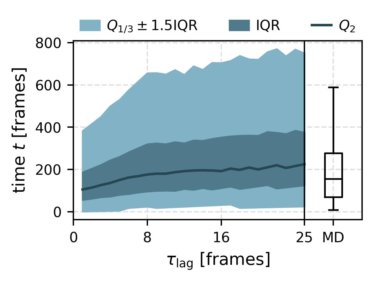
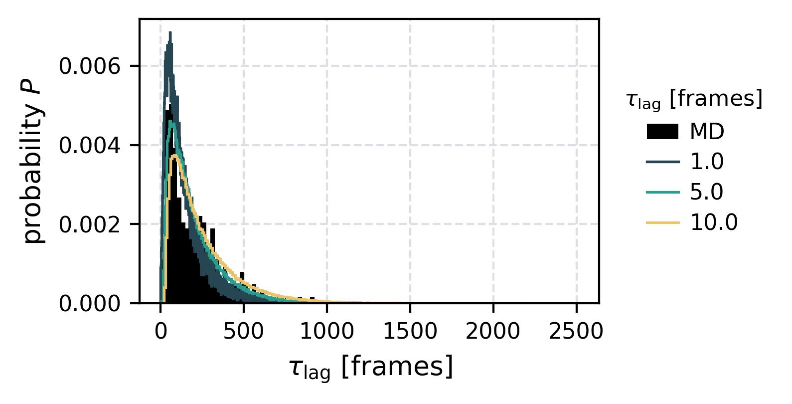
In the following we show some sample figures produced directly with the command line tools. For more information on that, there is a tutorial explaining the methods more in depth. In general we can see, that applying the HS-projection removes most projection artifacts based on coarse-graining many microstates into a few macrostates.

Method	MSM	Hummer-Szabo MSM
Implied Timescales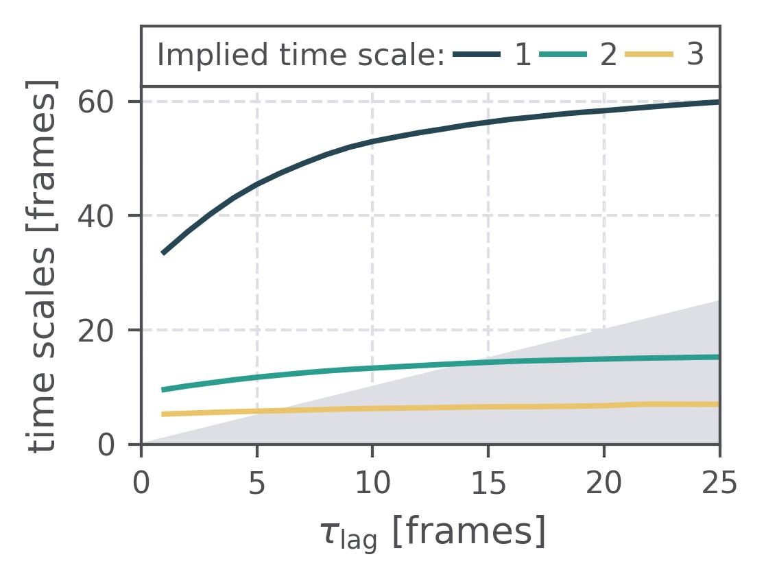
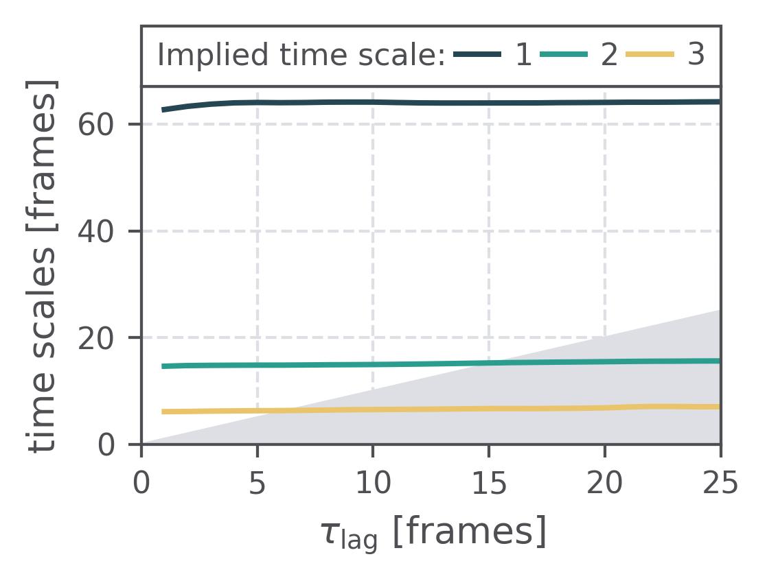Chapman-Kolmogorov test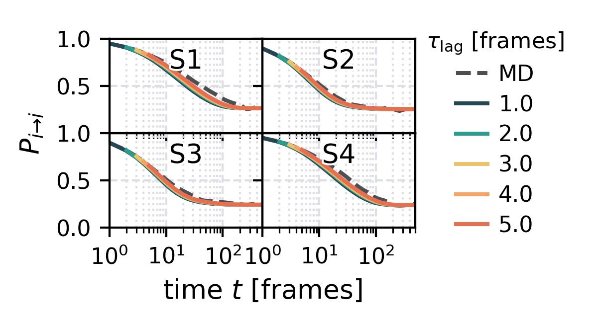
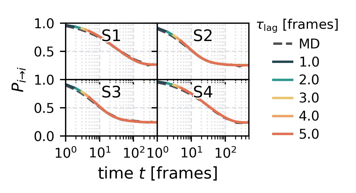Waiting Time Distributions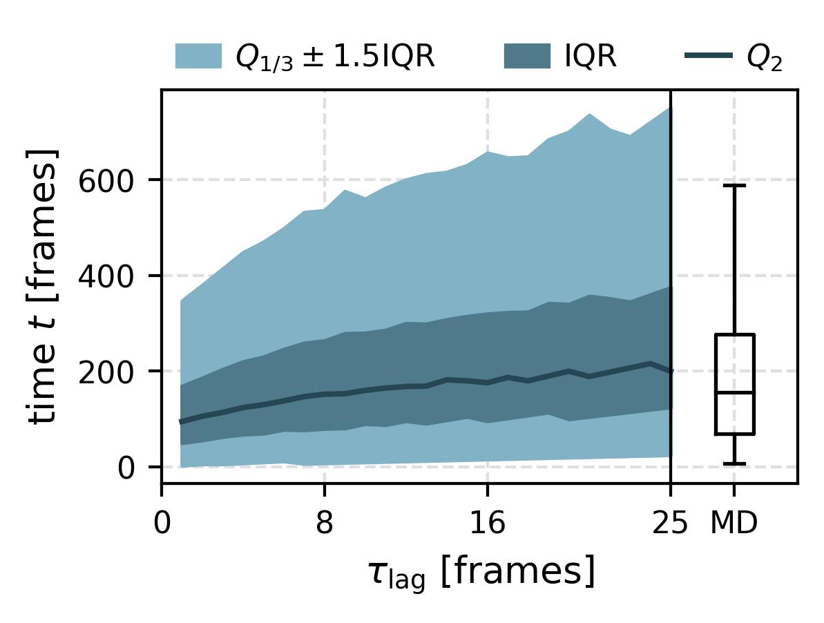
Waiting Times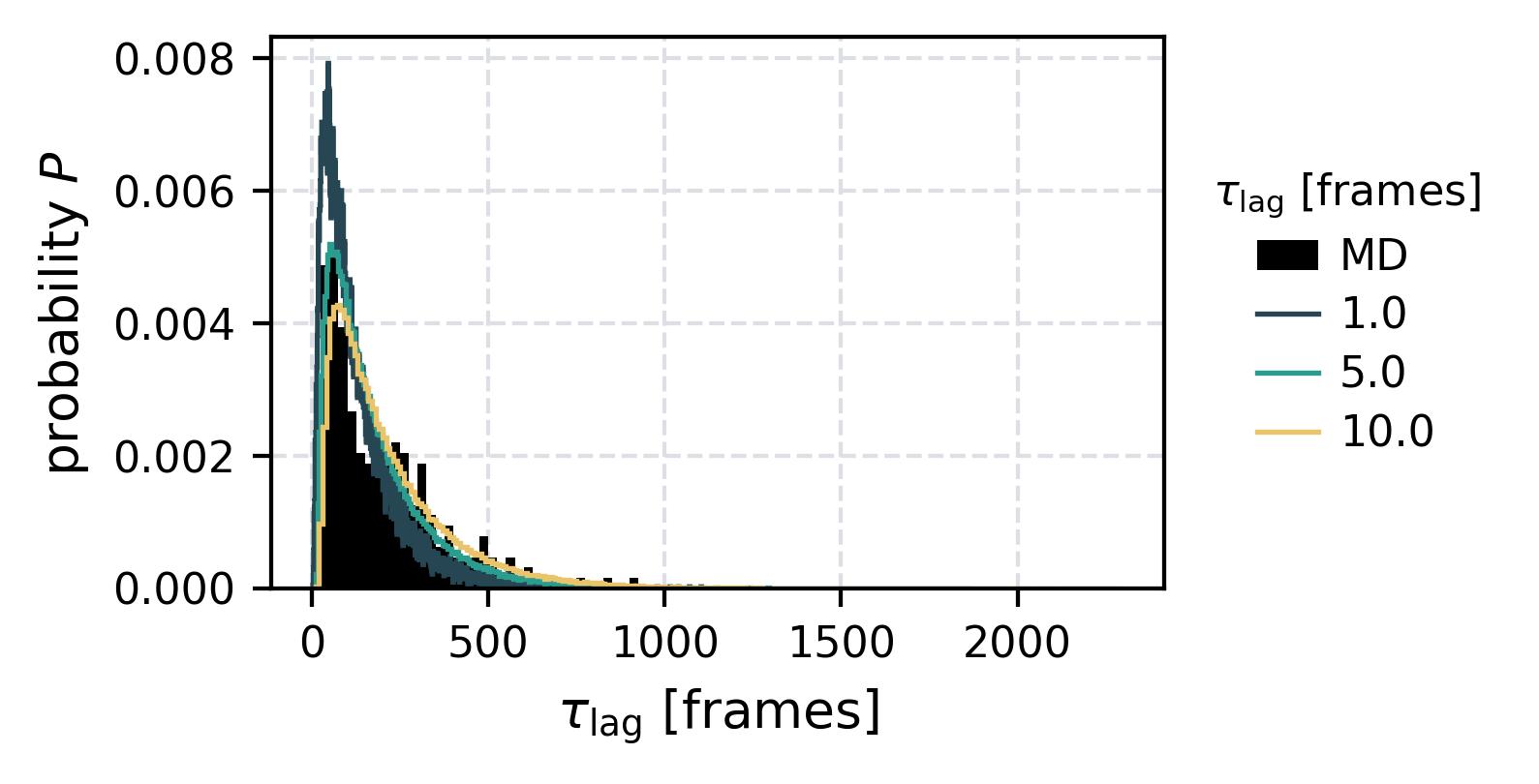
Contact Representation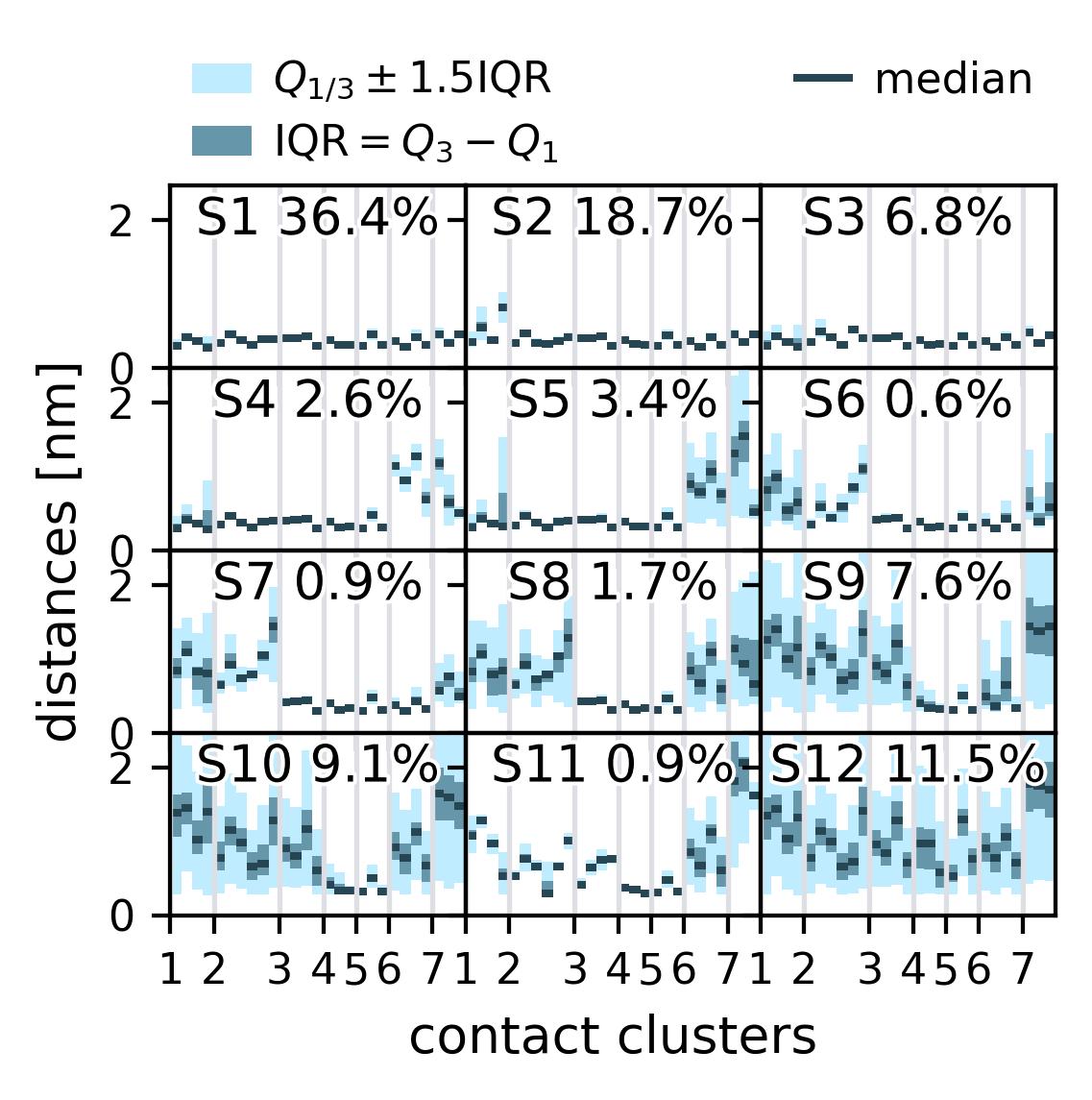

For more examples checkout the tutorials.

Roadmap

• Add Buchete-Hummer test as alternative for the Chapman-Kolmogorov test.
• Add a numba implementation of a parallelized autocorrelation function estimation.
• Use static type hints together with beartype